• 开源镜像
  • 开源沙龙
  • 媛宝
  • 猿帅
  • 注册
  • 登录
  • 息壤开源生活方式平台
  • 加入我们

开源日报

  • 2018年4月4日:开源日报第27期

    4 4 月, 2018

    每天推荐一个 GitHub 优质开源项目和一篇精选英文科技或编程文章原文,欢迎关注开源日报。交流QQ群:202790710;电报群 https://t.me/OpeningSourceOrg


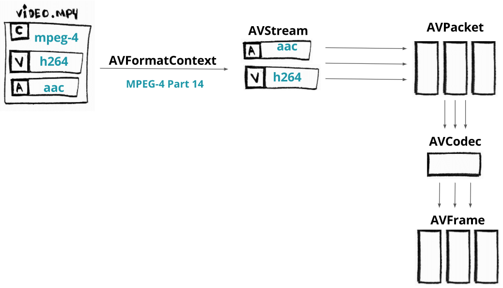
    今日推荐开源项目:《一个FFmpeg教程》

    推荐理由:FFmpeg 是一个非常优秀的视频处理开源工具,支持的格式和功能,可以说是非常齐全了。

    参数基本格式:

    作为一个命令行工具, FFmpeg 的参数按照如下格式输入:

    ffmpeg {1} {2} -i {3} {4} {5}

    1global options 全局选项

    2input file options 输入文件设置

    3input url 输入文件位置

    4output file options 输出文件设置

    5output url 输出文件位置


    正常使用的话只用记住这个:

    ffmpeg -i input.xxx {4} output.xxx

    4中内容有很多,可以选择编码器,声音处理,分辨率。帧率等等,常用的有这些:

    -s 分辨率(123×456这么写,要无损转换就填原视频分辨率)

    -aspect 视频长宽比(4:3, 16:9 or 1.3333, 1.7777)

    -an 取消音频

    -ac 设置声道数,1就是单声道,2就是立体声,转换单声道的TVrip可以用1(节省一半容量),高品质的DVDrip就可以用2

    例如:将一个1980×1080的mp4视频转化成同大小的avi,即输入:


    ffmpeg命令行工具指令集合:(来自http://blog.csdn.net/maopig/article/details/6610257)

    ffmpeg -i input.mp4 -s 1980×1080 output.avi


    基本选项:

    -formats 输出所有可用格式

    -f fmt     指定格式(音频或视频格式)

    -i filename    指定输入文件名,在linux下当然也能指定:0.0(屏幕录制)或摄像头

    -y    覆盖已有文件

    -t duration    记录时长为t

    -fs limit_size  设置文件大小上限

    -ss time_off   从指定的时间(s)开始, [-]hh:mm:ss[.xxx]的格式也支持

    -itsoffset time_off 设置时间偏移(s),该选项影响所有后面的输入文件。该偏移被加到输入文件的时戳,定义一个正偏移意味着相应的流被延迟了 offset秒。 [-]hh:mm:ss[.xxx]的格式也支持

    -title string    标题

    -timestamp time  时间戳

    -author string       作者

    -copyright string  版权信息

    -comment string  评论

    -album string album名

    -v verbose     与log相关的

    -target type   设置目标文件类型(“vcd”, “svcd”, “dvd”, “dv”, “dv50”, “pal-vcd”, “ntsc-svcd”, …)

    -dframes number 设置要记录的帧数


    视频选项:

    -b   指定比特率(bits/s),似乎FFmpeg是自动VBR的,指定了就大概是平均比特率

    -bitexact 使用标准比特率

    -vb  指定视频比特率(bits/s)

    -vframes number  设置转换多少桢(frame)的视频

    -r rate    帧速率(fps) (可以改,确认非标准桢率会导致音画不同步,所以只能设定为15或者29.97)

    -s size    指定分辨率 (320×240)

    -aspect aspect      设置视频长宽比(4:3, 16:9 or 1.3333, 1.7777)

    -croptop size 设置顶部切除尺寸(in pixels)

    -cropbottom size  设置底部切除尺寸(in pixels)

    -cropleft size 设置左切除尺寸 (in pixels)

    -cropright size      设置右切除尺寸 (in pixels)

    -padtop size  设置顶部补齐尺寸(in pixels)

    -padbottom size   底补齐(in pixels)

    -padleft size  左补齐(in pixels)

    -padright size       右补齐(in pixels)

    -padcolor color    补齐带颜色(000000-FFFFFF)

    -vn  取消视频

    -vcodec codec      强制使用codec编解码方式(‘copy’ to copy stream)

    -sameq  使用同样视频质量作为源(VBR)

    -pass n   选择处理遍数(1或者2)。两遍编码非常有用。第一遍生成统计信息,第二遍生成精确的请求的码率

    -passlogfile file     选择两遍的纪录文件名为file

    -newvideo     在现在的视频流后面加入新的视频流


    高级视频选项:

    -pix_fmt format    set pixel format, ‘list’ as argument shows all the pixel formats supported

    -intra     仅适用帧内编码

    -qscale q       以<数值>质量为基础的VBR,取值0.01-255,约小质量越好

    -loop_input   设置输入流的循环数(目前只对图像有效)

    -loop_output 设置输出视频的循环数,比如输出gif时设为0表示无限循环

    -g int     设置图像组大小

    -cutoff int      设置截止频率

    -qmin int       设定最小质量,与-qmax(设定最大质量)共用,比如-qmin 10 -qmax 31

    -qmax int      设定最大质量

    -qdiff int 量化标度间最大偏差 (VBR)

    -bf int    使用frames B 帧,支持mpeg1,mpeg2,mpeg4


    音频选项:

    -ab 设置比特率(单位:bit/s,也许老版是kb/s)前面-ac设为立体声时要以一半比特率来设置,比如192kbps的就设成96,转换 默认比特率都较小,要听到较高品质声音的话建议设到160kbps(80)以上。

    -aframes number 设置转换多少桢(frame)的音频

    -aq quality    设置音频质量 (指定编码)

    -ar rate  设置音频采样率 (单位:Hz),PSP只认24000

    -ac channels 设置声道数,1就是单声道,2就是立体声,转换单声道的TVrip可以用1(节省一半容量),高品质的DVDrip就可以用2

    -an 取消音频

    -acodec codec     指定音频编码(‘copy’ to copy stream)

    -vol volume   设置录制音量大小(默认为256) <百分比> ,某些DVDrip的AC3轨音量极小,转换时可以用这个提高音量,比如200就是原来的2倍

    -newaudio    在现在的音频流后面加入新的音频流


    字幕选项:

    -sn  取消字幕

    -scodec codec      设置字幕编码(‘copy’ to copy stream)

    -newsubtitle  在当前字幕后新增

    -slang code   设置字幕所用的ISO 639编码(3个字母)

    Audio/Video 抓取选项:

    -vc channel   设置视频捕获通道(只对DV1394)

    -tvstd standard     设置电视标准 NTSC PAL(SECAM)


    音频转换:

    要得到一个高画质音质低容量的MP4的话,首先画面最好不要用固定比特率,而用VBR参数让程序自己去判断,而音质参数可以在原来的基础上提升一点,听起来要舒服很多,也不会太大(看情况调整 )


    转换为flv:

    ffmpeg -i test.mp3 -ab 56 -ar 22050 -b 500 -r 15 -s 320×240 test.flv

    ffmpeg -i test.wmv -ab 56 -ar 22050 -b 500 -r 15 -s 320×240 test.flv


    转换文件格式的同时抓缩微图:

    ffmpeg -i “test.avi” -y -f image2 -ss 8 -t 0.001 -s 350×240 ‘test.jpg’


    对已有flv抓图:

    ffmpeg -i “test.flv” -y -f image2 -ss 8 -t 0.001 -s 350×240 ‘test.jpg’


    转换为3gp:

    ffmpeg -y -i test.mpeg -bitexact -vcodec h263 -b 128 -r 15 -s 176×144 -acodec aac -ac 2 -ar 22500 -ab 24 -f 3gp test.3gp

    ffmpeg -y -i test.mpeg -ac 1 -acodec amr_nb -ar 8000 -s 176×144 -b 128 -r 15 test.3gp


    参数解释:

    -y(覆盖输出文件,即如果1.***文件已经存在的话,不经提示就覆盖掉了)

    -i “1.avi”(输入文件是和ffmpeg在同一目录下的1.avi文件,可以自己加路径,改名字)

    -title “Test”(在PSP中显示的影片的标题)

    -vcodec xvid(使用XVID编码压缩视频,不能改的)

    -s 368×208(输出的分辨率为368×208,注意片源一定要是16:9的不然会变形)

    -r 29.97(帧数,一般就用这个吧)

    -b 1500(视频数据流量,用-b xxxx的指令则使用固定码率,数字随便改,1500以上没效果;还可以用动态码率如:-qscale 4和-qscale 6,4的质量比6高)

    -acodec aac(音频编码用AAC)

    -ac 2(声道数1或2)

    -ar 24000(声音的采样频率,好像PSP只能支持24000Hz)

    -ab 128(音频数据流量,一般选择32、64、96、128)

    -vol 200(200%的音量,自己改)

    -f psp(输出psp专用格式)

    -muxvb 768(好像是给PSP机器识别的码率,一般选择384、512和768,我改成1500,PSP就说文件损坏了)

    “test.***”(输出文件名,也可以加路径改文件名)


    今日推荐英文原文:《Introducing TensorFlow.js: Machine Learning in Javascript》作者:Josh Gordon / Sara Robinson

    原文链接:https://medium.com/tensorflow/introducing-tensorflow-js-machine-learning-in-javascript-bf3eab376db

    推荐理由:关注人工智能的同学想必都知道 TensorFlow,然而不一定知道 TensorFlow.js 吧?这是一个可以使用 JavaScript 在你的浏览器运行的人工智能 API,如果你是一个前端开发者,又对机器学习感兴趣,那么这是一个非常棒的学习的开始。

    Introducing TensorFlow.js: Machine Learning in Javascript

    We’re excited to introduce TensorFlow.js, an open-source library you can use to define, train, and run machine learning models entirely in the browser, using Javascript and a high-level layers API. If you’re a Javascript developer who’s new to ML, TensorFlow.js is a great way to begin learning. Or, if you’re a ML developer who’s new to Javascript, read on to learn more about new opportunities for in-browser ML. In this post, we’ll give you a quick overview of TensorFlow.js, and getting started resources you can use to try it out.

    In-Browser ML

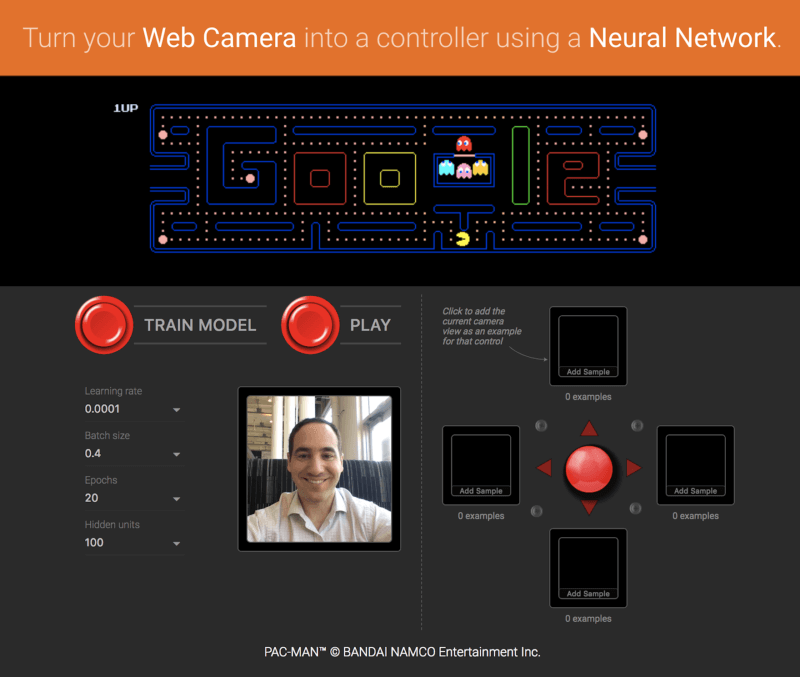
    Running machine learning programs entirely client-side in the browser unlocks new opportunities, like interactive ML! If you’re watching the livestream for the TensorFlow Developer Summit, during the TensorFlow.js talk you’ll find a demo where @dsmilkov and @nsthorat train a model to control a PAC-MAN game using computer vision and a webcam, entirely in the browser. You can try it out yourself, too, with the link below — and find the source in the examples folder.

     
    Turn your webcam into a controller for PAC-MAN using a Neural Network.

    If you’d like to try another game, give the Emoji Scavenger Hunt a whirl — this time, from a browser on your mobile phone.

     
    The Emoji Scavenger Hunt is another fun example of an application built using TensorFlow.js. Try it using your phone, and find the source here.

    ML running in the browser means that from a user’s perspective, there’s no need to install any libraries or drivers. Just open a webpage, and your program is ready to run. In addition, it’s ready to run with GPU acceleration. TensorFlow.js automatically supports WebGL, and will accelerate your code behind the scenes when a GPU is available. Users may also open your webpage from a mobile device, in which case your model can take advantage of sensor data, say from a gyroscope or accelerometer. Finally, all data stays on the client, making TensorFlow.js useful for low-latency inference, as well as for privacy preserving applications.

    What can you do with TensorFlow.js?

    If you’re developing with TensorFlow.js, here are three workflows you can consider.

    • You can import an existing, pre-trained model for inference. If you have an existing TensorFlow or Keras model you’ve previously trained offline, you can convert into TensorFlow.js format, and load it into the browser for inference.
    • You can re-train an imported model. As in the Pac-Man demo above, you can use transfer learning to augment an existing model trained offline using a small amount of data collected in the browser using a technique called Image Retraining. This is one way to train an accurate model quickly, using only a small amount of data.
    • Author models directly in browser. You can also use TensorFlow.js to define, train, and run models entirely in the browser using Javascript and a high-level layers API. If you’re familiar with Keras, the high-level layers API should feel familiar.

    Let’s see some code

    If you like, you can head directly to the samples or tutorials to get started. These show how-to export a model defined in Python for inference in the browser, as well as how to define and train models entirely in Javascript. As a quick preview, here’s a snippet of code that defines a neural network to classify flowers, much like on the getting started guide on TensorFlow.org. Here, we’ll define a model using a stack of layers.

    import * as tf from ‘@tensorflow/tfjs’;
    const model = tf.sequential();
    model.add(tf.layers.dense({inputShape: [4], units: 100}));
    model.add(tf.layers.dense({units: 4}));
    model.compile({loss: ‘categoricalCrossentropy’, optimizer: ‘sgd’});

    The layers API we’re using here supports all of the Keras layers found in the examples directory (including Dense, CNN, LSTM, and so on). We can then train our model using the same Keras-compatible API with a method call:

    await model.fit(
      xData, yData, {
        batchSize: batchSize,
        epochs: epochs
    });

    The model is now ready to use to make predictions:

    // Get measurements for a new flower to generate a prediction
    // The first argument is the data, and the second is the shape.
    const inputData = tf.tensor2d([[4.8, 3.0, 1.4, 0.1]], [1, 4]);
    
    // Get the highest confidence prediction from our model
    const result = model.predict(inputData);
    const winner = irisClasses[result.argMax().dataSync()[0]];
    
    // Display the winner
    console.log(winner);

    TensorFlow.js also includes a low-level API (previously deeplearn.js) and support for Eager execution. You can learn more about these by watching the talk at the TensorFlow Developer Summit.

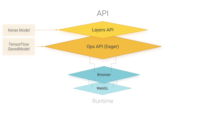
    An overview of TensorFlow.js APIs. TensorFlow.js is powered by WebGL and provides a high-level layers API for defining models, and a low-level API for linear algebra and automatic differentiation. TensorFlow.js supports importing TensorFlow SavedModels and Keras models.

    How does TensorFlow.js relate to deeplearn.js?

    Good question! TensorFlow.js, an ecosystem of JavaScript tools for machine learning, is the successor to deeplearn.js which is now called TensorFlow.js Core. TensorFlow.js also includes a Layers API, which is a higher level library for building machine learning models that uses Core, as well as tools for automatically porting TensorFlow SavedModels and Keras hdf5 models. For answers to more questions like this, check out the FAQ.


    每天推荐一个 GitHub 优质开源项目和一篇精选英文科技或编程文章原文,欢迎关注开源日报。交流QQ群:202790710;电报群 https://t.me/OpeningSourceOrg

  • 2018年4月3日:开源日报第26期

    3 4 月, 2018

    每天推荐一个 GitHub 优质开源项目和一篇精选英文科技或编程文章原文,欢迎关注开源日报。交流QQ群:202790710;电报群 https://t.me/OpeningSourceOrg


    今日推荐开源项目:《网页动画特效框架Micron.js》

    推荐理由:Micron.js是一个能够为元素添加css动画效果的js库,目前有12种特效,可以自己设定动画时间的长短,也可实现动画的绑定效果,通过点击一个元素控制另一个元素。

    安装:

    要在自己的html文件中使用micron.js有两种方法:

    1.在head标签中加入:

    <link href="https://unpkg.com/[email protected]/dist/css/micron.min.css" type="text/css" rel="stylesheet">
    <script src="https://unpkg.com/[email protected]/dist/script/micron.min.js" type="text/javascript"></script>

    直接通过链接导入micron.js

    2.本地安装micron.js

    使用npm:npm install webkul-micron

    使用bower:bower install webkul-micron

    安装完后在html中导入本地文件中的micron.min.css和micron.min.js就可以使用micron.js添加自己想要的特效

    添加特效:

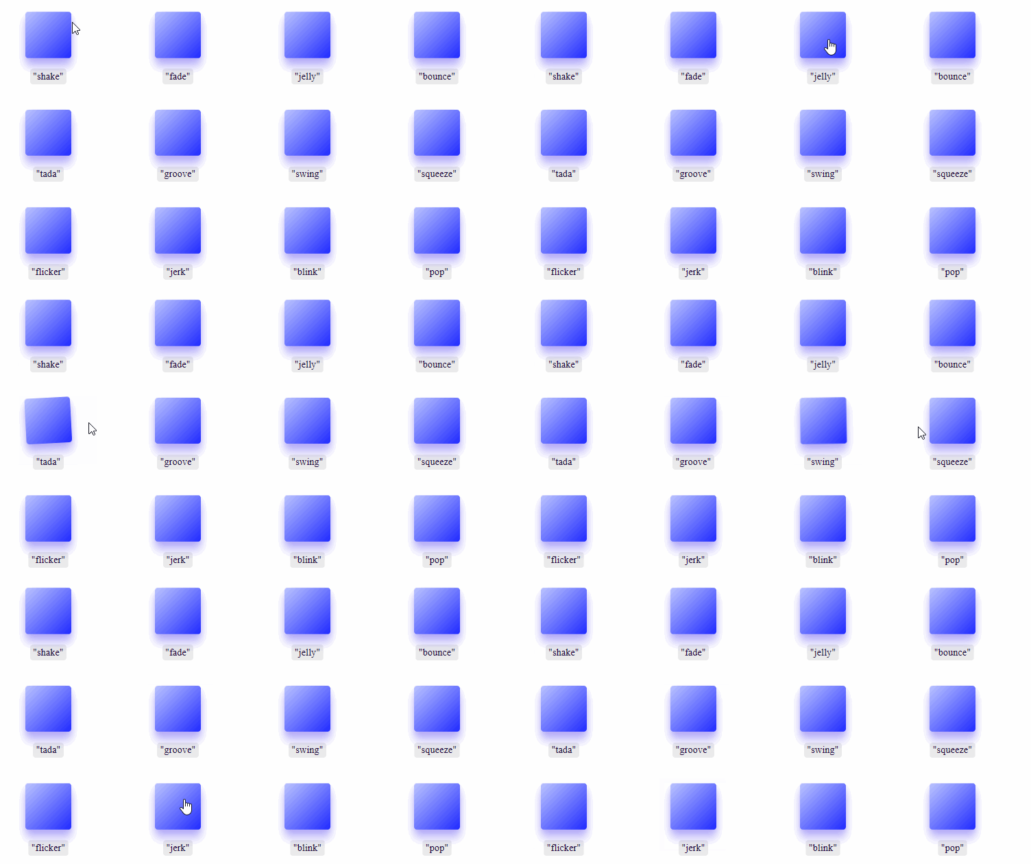
    使用micron.js十分简单,只需在想添加动画特效的元素标签中写data-micron=”XXX”(XXX为想添加的特效的名称),目前mircron.js支持12种特效:shake,fade,jelly,bounce,tada,groove,swing,squeeze,flicker,jerk,blink,pop.

    特效演示:

    播放时间设置:

    在添加了动画特效的元素标签中添加data-micron-duration=”XXX”(XXX为播放时间,以秒为单位) , 如data-micron-duration=”.95″代表将播放时间设置为0.95s,如果没有设置,默认值为0.45s

    效果演示:

    绑定效果设置:

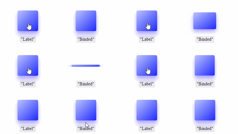
    添加绑定效果需要在施加控制的元素中除了设置特效外,还需设置data-micron-bind的为true,并通过data-micron-id 设置受控制元素的id

    如

    <a href="#!" class="button" data-micron="bounce" data-micron-bind="true" data-micron-id="me">Label</a> 
    <a href="#!" class="button" id="me">Binded</a>

    点击Label元素id为”me”的元素就会产生bounce特效效果演示:


    链接:

    https://github.com/webkul/micron


    今日推荐英文原文:《Understanding Linux filesystems: ext4 and beyond》原作者:Jim Salter

    原文链接:https://opensource.com/article/18/4/ext4-filesystem

    推荐理由:大多数 Linux 发行版默认使用的文件系统都是 ext4,之前是 ext3,那么 ext4 文件系统有哪些特点呢?它的历史演变是怎样?跟别的文件系统有什么优劣不同?看这一篇文章就都清楚了。

    Understanding Linux filesystems: ext4 and beyond

    People work on a computer server
    Image by :opensource.com

    The majority of modern Linux distributions default to the ext4 filesystem, just as previous Linux distributions defaulted to ext3, ext2, and—if you go back far enough—ext.

    If you’re new to Linux—or to filesystems—you might wonder what ext4 brings to the table that ext3 didn’t. You might also wonder whether ext4 is still in active development at all, given the flurries of news coverage of alternate filesystems such as btrfs, xfs, and zfs.

    We can’t cover everything about filesystems in a single article, but we’ll try to bring you up to speed on the history of Linux’s default filesystem, where it stands, and what to look forward to.I drew heavily on Wikipedia’s various ext filesystem articles, kernel.org’s wiki entries on ext4, and my own experiences while preparing this overview.

    A brief history of ext

    MINIX filesystem

    Before there was ext, there was the MINIX filesystem. If you’re not up on your Linux history, MINIX was a very small Unix-like operating system for IBM PC/AT microcomputers. Andrew Tannenbaum developed it for teaching purposes and released its source code (in print form!) in 1987.

    IBM PC AT

    IBM’s mid-1980s PC/AT, MBlairMartin, CC BY-SA 4.0

    Although you could peruse MINIX’s source, it was not actually free and open source software (FOSS). The publishers of Tannebaum’s book required a $69 license fee to operate MINIX, which was included in the cost of the book. Still, this was incredibly inexpensive for the time, and MINIX adoption took off rapidly, soon exceeding Tannenbaum’s original intent of using it simply to teach the coding of operating systems. By and throughout the 1990s, you could find MINIX installations thriving in universities worldwide—and a young Linus Torvalds used MINIX to develop the original Linux kernel, first announced in 1991, and released under the GPL in December 1992.

    But wait, this is a filesystem article, right? Yes, and MINIX had its own filesystem, which early versions of Linux also relied on. Like MINIX, it could uncharitably be described as a “toy” example of its kind—the MINIX filesystem could handle filenames only up to 14 characters and address only 64MB of storage. In 1991, the typical hard drive was already 40-140MB in size. Linux clearly needed a better filesystem!

    ext

    While Linus hacked away on the fledgling Linux kernel, Rémy Card worked on the first ext filesystem. First implemented in 1992—only a year after the initial announcement of Linux itself!—ext solved the worst of the MINIX filesystem’s problems.

    1992’s ext used the new virtual filesystem (VFS) abstraction layer in the Linux kernel. Unlike the MINIX filesystem before it, ext could address up to 2GB of storage and handle 255-character filenames.

    But ext didn’t have a long reign, largely due to its primitive timestamping (only one timestamp per file, rather than the three separate stamps for inode creation, file access, and file modification we’re familiar with today). A mere year later, ext2 ate its lunch.

    ext2

    Rémy clearly realized ext’s limitations pretty quickly, since he designed ext2 as its replacement a year later. While ext still had its roots in “toy” operating systems, ext2 was designed from the start as a commercial-grade filesystem, along the same principles as BSD’s Berkeley Fast File System.

    Ext2 offered maximum filesizes in the gigabytes and filesystem sizes in the terabytes, placing it firmly in the big leagues for the 1990s. It was quickly and widely adopted, both in the Linux kernel and eventually in MINIX, as well as by third-party modules making it available for MacOS and Windows.

    There were still problems to solve, though: ext2 filesystems, like most filesystems of the 1990s, were prone to catastrophic corruption if the system crashed or lost power while data was being written to disk. They also suffered from significant performance losses due to fragmentation (the storage of a single file in multiple places, physically scattered around a rotating disk) as time went on.

    Despite these problems, ext2 is still used in some isolated cases today—most commonly, as a format for portable USB thumb drives.

    ext3

    In 1998, six years after ext2’s adoption, Stephen Tweedie announced he was working on significantly improving it. This became ext3, which was adopted into mainline Linux with kernel version 2.4.15, in November 2001.

    Packard Bell computer

    Mid-1990s Packard Bell computer, Spacekid, CC0

    Ext2 had done very well by Linux distributions for the most part, but—like FAT, FAT32, HFS, and other filesystems of the time—it was prone to catastrophic corruption during power loss. If you lose power while writing data to the filesystem, it can be left in what’s called an inconsistent state—one in which things have been left half-done and half-undone. This can result in loss or corruption of vast swaths of files unrelated to the one being saved or even unmountability of the entire filesystem.

    Ext3, and other filesystems of the late 1990s, such as Microsoft’s NTFS, uses journaling to solve this problem. The journal is a special allocation on disk where writes are stored in transactions; if the transaction finishes writing to disk, its data in the journal is committed to the filesystem itself. If the system crashes before that operation is committed, the newly rebooted system recognizes it as an incomplete transaction and rolls it back as though it had never taken place. This means that the file being worked on may still be lost, but the filesystem itself remains consistent, and all other data is safe. Three levels of journaling are available in the Linux kernel implementation of ext3: journal, ordered, and writeback.

    • Journal is the lowest risk mode, writing both data and metadata to the journal before committing it to the filesystem. This ensures consistency of the file being written to, as well as the filesystem as a whole, but can significantly decrease performance.
    • Ordered is the default mode in most Linux distributions; ordered mode writes metadata to the journal but commits data directly to the filesystem. As the name implies, the order of operations here is rigid: First, metadata is committed to the journal; second, data is written to the filesystem, and only then is the associated metadata in the journal flushed to the filesystem itself. This ensures that, in the event of a crash, the metadata associated with incomplete writes is still in the journal, and the filesystem can sanitize those incomplete writes while rolling back the journal. In ordered mode, a crash may result in corruption of the file or files being actively written to during the crash, but the filesystem itself—and files not actively being written to—are guaranteed safe.
    • Writeback is the third—and least safe—journaling mode. In writeback mode, like ordered mode, metadata is journaled, but data is not. Unlike ordered mode, metadata and data alike may be written in whatever order makes sense for best performance. This can offer significant increases in performance, but it’s much less safe. Although writeback mode still offers a guarantee of safety to the filesystem itself, files that were written to during or before the crash are vulnerable to loss or corruption.

    Like ext2 before it, ext3 uses 16-bit internal addressing. This means that with a blocksize of 4K, the largest filesize it can handle is 2 TiB in a maximum filesystem size of 16 TiB.

    ext4

    Theodore Ts’o (who by then was ext3’s principal developer) announced ext4 in 2006, and it was added to mainline Linux two years later, in kernel version 2.6.28. Ts’o describes ext4 as a stopgap technology which significantly extends ext3 but is still reliant on old technology. He expects it to be supplanted eventually by a true next-generation filesystem.

    Dell Precision 380 workstation

    Dell Precision 380 workstation, Lance Fisher, CC BY-SA 2.0

    Ext4 is functionally very similar to ext3, but brings large filesystem support, improved resistance to fragmentation, higher performance, and improved timestamps.

    Ext4 vs ext3

    Ext3 and ext4 have some very specific differences, which I’ll focus on here.

    Backwards compatibility

    Ext4 was specifically designed to be as backward-compatible as possible with ext3. This not only allows ext3 filesystems to be upgraded in place to ext4; it also permits the ext4 driver to automatically mount ext3 filesystems in ext3 mode, making it unnecessary to maintain the two codebases separately.

    Large filesystems

    Ext3 filesystems used 32-bit addressing, limiting them to 2 TiB files and 16 TiB filesystems (assuming a 4 KiB blocksize; some ext3 filesystems use smaller blocksizes and are thus limited even further).

    Ext4 uses 48-bit internal addressing, making it theoretically possible to allocate files up to 16 TiB on filesystems up to 1,000,000 TiB (1 EiB). Early implementations of ext4 were still limited to 16 TiB filesystems by some userland utilities, but as of 2011, e2fsprogs has directly supported the creation of >16TiB ext4 filesystems. As one example, Red Hat Enterprise Linux contractually supports ext4 filesystems only up to 50 TiB and recommends ext4 volumes no larger than 100 TiB.

    Allocation improvements

    Ext4 introduces a lot of improvements in the ways storage blocks are allocated before writing them to disk, which can significantly increase both read and write performance.

    Extents

    An extent is a range of contiguous physical blocks (up to 128 MiB, assuming a 4 KiB block size) that can be reserved and addressed at once. Utilizing extents decreases the number of inodes required by a given file and significantly decreases fragmentation and increases performance when writing large files.

    Multiblock allocation

    Ext3 called its block allocator once for each new block allocated. This could easily result in heavy fragmentation when multiple writers are open concurrently. However, ext4 uses delayed allocation, which allows it to coalesce writes and make better decisions about how to allocate blocks for the writes it has not yet committed.

    Persistent pre-allocation

    When pre-allocating disk space for a file, most file systems must write zeroes to the blocks for that file on creation. Ext4 allows the use of fallocate() instead, which guarantees the availability of the space (and attempts to find contiguous space for it) without first needing to write to it. This significantly increases performance in both writes and future reads of the written data for streaming and database applications.

    Delayed allocation

    This is a chewy—and contentious—feature. Delayed allocation allows ext4 to wait to allocate the actual blocks it will write data to until it’s ready to commit that data to disk. (By contrast, ext3 would allocate blocks immediately, even while the data was still flowing into a write cache.)

    Delaying allocation of blocks as data accumulates in cache allows the filesystem to make saner choices about how to allocate those blocks, reducing fragmentation (write and, later, read) and increasing performance significantly. Unfortunately, it increases the potential for data loss in programs that have not been specifically written to call fsync() when the programmer wants to ensure data has been flushed entirely to disk.

    Let’s say a program rewrites a file entirely:

    fd=open("file" ,O_TRUNC); write(fd, data); close(fd);

    With legacy filesystems, close(fd); is sufficient to guarantee that the contents of file will be flushed to disk. Even though the write is not, strictly speaking, transactional, there’s very little risk of losing the data if a crash occurs after the file is closed.

    If the write does not succeed (due to errors in the program, errors on the disk, power loss, etc.), both the original version and the newer version of the file may be lost or corrupted. If other processes access the file as it is being written, they will see a corrupted version. And if other processes have the file open and do not expect its contents to change—e.g., a shared library mapped into multiple running programs—they may crash.

    To avoid these issues, some programmers avoid using O_TRUNC at all. Instead, they might write to a new file, close it, then rename it over the old one:

    fd=open("newfile"); write(fd, data); close(fd); rename("newfile", "file");

    Under filesystems without delayed allocation, this is sufficient to avoid the potential corruption and crash problems outlined above: Since rename() is an atomic operation, it won’t be interrupted by a crash; and running programs will continue to reference the old, now unlinked version of file for as long as they have an open filehandle to it. But because ext4’s delayed allocation can cause writes to be delayed and re-ordered, the rename("newfile","file") may be carried out before the contents of newfile are actually written to disk, which opens the problem of parallel processes getting bad versions of file all over again.

    To mitigate this, the Linux kernel (since version 2.6.30) attempts to detect these common code cases and force the files in question to be allocated immediately. This reduces, but does not prevent, the potential for data loss—and it doesn’t help at all with new files. If you’re a developer, please take note: The only way to guarantee data is written to disk immediately is to call fsync() appropriately.

    Unlimited subdirectories

    Ext3 was limited to a total of 32,000 subdirectories; ext4 allows an unlimited number. Beginning with kernel 2.6.23, ext4 uses HTree indices to mitigate performance loss with huge numbers of subdirectories.

    Journal checksumming

    Ext3 did not checksum its journals, which presented problems for disk or controller devices with caches of their own, outside the kernel’s direct control. If a controller or a disk with its own cache did writes out of order, it could break ext3’s journaling transaction order, potentially corrupting files being written to during (or for some time preceding) a crash.

    In theory, this problem is resolved by the use of write barriers—when mounting the filesystem, you set barrier=1 in the mount options, and the device will then honor fsync() calls all the way down to the metal. In practice, it’s been discovered that storage devices and controllers frequently do not honor write barriers—improving performance (and benchmarks, where they’re compared to their competitors) but opening up the possibility of data corruption that should have been prevented.

    Checksumming the journal allows the filesystem to realize that some of its entries are invalid or out-of-order on the first mount after a crash. This thereby avoids the mistake of rolling back partial or out-of-order journal entries and further damaging the filesystem—even if the storage devices lie and don’t honor barriers.

    Fast filesystem checks

    Under ext3, the entire filesystem—including deleted and empty files—required checking when fsck is invoked. By contrast, ext4 marks unallocated blocks and sections of the inode table as such, allowing fsck to skip them entirely. This greatly reduces the time to run fsck on most filesystems and has been implemented since kernel 2.6.24.

    Improved timestamps

    Ext3 offered timestamps granular to one second. While sufficient for most uses, mission-critical applications are frequently looking for much, much tighter time control. Ext4 makes itself available to those enterprise, scientific, and mission-critical applications by offering timestamps in the nanoseconds.

    Ext3 filesystems also did not provide sufficient bits to store dates beyond January 18, 2038. Ext4 adds an additional two bits here, extending the Unix epoch another 408 years. If you’re reading this in 2446 AD, you have hopefully already moved onto a better filesystem—but it’ll make me posthumously very, very happy if you’re still measuring the time since UTC 00:00, January 1, 1970.

    Online defragmentation

    Neither ext2 nor ext3 directly supported online defragmentation—that is, defragging the filesystem while mounted. Ext2 had an included utility, e2defrag, that did what the name implies—but it needed to be run offline while the filesystem was not mounted. (This is, obviously, especially problematic for a root filesystem.) The situation was even worse in ext3—although ext3 was much less likely to suffer from severe fragmentation than ext2 was, running e2defrag against an ext3 filesystem could result in catastrophic corruption and data loss.

    Although ext3 was originally deemed “unaffected by fragmentation,” processes that employ massively parallel write processes to the same file (e.g., BitTorrent) made it clear that this wasn’t entirely the case. Several userspace hacks and workarounds, such as Shake, addressed this in one way or another—but they were slower and in various ways less satisfactory than a true, filesystem-aware, kernel-level defrag process.

    Ext4 addresses this problem head on with e4defrag, an online, kernel-mode, filesystem-aware, block-and-extent-level defragmentation utility.

    Ongoing ext4 development

    Ext4 is, as the Monty Python plague victim once said, “not quite dead yet!” Although its principal developer regards it as a mere stopgap along the way to a truly next-generation filesystem, none of the likely candidates will be ready (due to either technical or licensing problems) for deployment as a root filesystem for some time yet.

    There are still a few key features being developed into future versions of ext4, including metadata checksumming, first-class quota support, and large allocation blocks.

    Metadata checksumming

    Since ext4 has redundant superblocks, checksumming the metadata within them offers the filesystem a way to figure out for itself whether the primary superblock is corrupt and needs to use an alternate. It is possible to recover from a corrupt superblock without checksumming—but the user would first need to realize that it was corrupt, and then try manually mounting the filesystem using an alternate. Since mounting a filesystem read-write with a corrupt primary superblock can, in some cases, cause further damage, this isn’t a sufficient solution, even with a sufficiently experienced user!

    Compared to the extremely robust per-block checksumming offered by next-gen filesystems such as btrfs or zfs, ext4’s metadata checksumming is a pretty weak feature. But it’s much better than nothing.

    Although it sounds like a no-brainer—yes, checksum ALL THE THINGS!—there are some significant challenges to bolting checksums into a filesystem after the fact; see the design document for the gritty details.

    First-class quota support

    Wait, quotas?! We’ve had those since the ext2 days! Yes, but they’ve always been an afterthought, and they’ve always kinda sucked. It’s probably not worth going into the hairy details here, but the design document lays out the ways quotas will be moved from userspace into the kernel and more correctly and performantly enforced.

    Large allocation blocks

    As time goes by, those pesky storage systems keep getting bigger and bigger. With some solid-state drives already using 8K hardware blocksizes, ext4’s current limitation to 4K blocks gets more and more limiting. Larger storage blocks can decrease fragmentation and increase performance significantly, at the cost of increased “slack” space (the space left over when you only need part of a block to store a file or the last piece of a file).

    You can view the hairy details in the design document.

    Practical limitations of ext4

    Ext4 is a robust, stable filesystem, and it’s what most people should probably be using as a root filesystem in 2018. But it can’t handle everything. Let’s talk briefly about some of the things you shouldn’t expect from ext4—now or probably in the future.

    Although ext4 can address up to 1 EiB—equivalent to 1,000,000 TiB—of data, you really, really shouldn’t try to do so. There are problems of scale above and beyond merely being able to remember the addresses of a lot more blocks, and ext4 does not now (and likely will not ever) scale very well beyond 50-100 TiB of data.

    Ext4 also doesn’t do enough to guarantee the integrity of your data. As big an advancement as journaling was back in the ext3 days, it does not cover a lot of the common causes of data corruption. If data is corrupted while already on disk—by faulty hardware, impact of cosmic rays (yes, really), or simple degradation of data over time—ext4 has no way of either detecting or repairing such corruption.

    Building on the last two items, ext4 is only a pure filesystem, and not a storage volume manager. This means that even if you’ve got multiple disks—and therefore parity or redundancy, which you could theoretically recover corrupt data from—ext4 has no way of knowing that or using it to your benefit. While it’s theoretically possible to separate a filesystem and storage volume management system in discrete layers without losing automatic corruption detection and repair features, that isn’t how current storage systems are designed, and it would present significant challenges to new designs.

    Alternate filesystems

    Before we get started, a word of warning: Be very careful with any alternate filesystem which isn’t built into and directly supported as a part of your distribution’s mainline kernel!

    Even if a filesystem is safe, using it as the root filesystem can be absolutely terrifying if something hiccups during a kernel upgrade. If you aren’t extremely comfortable with the idea of booting from alternate media and poking manually and patiently at kernel modules, grub configs, and DKMS from a chroot… don’t go off the reservation with the root filesystem on a system that matters to you.

    There may well be good reasons to use a filesystem your distro doesn’t directly support—but if you do, I strongly recommend you mount it after the system is up and usable. (For example, you might have an ext4 root filesystem, but store most of your data on a zfs or btrfs pool.)

    XFS

    XFS is about as mainline as a non-ext filesystem gets under Linux. It’s a 64-bit, journaling filesystem that has been built into the Linux kernel since 2001 and offers high performance for large filesystems and high degrees of concurrency (i.e., a really large number of processes all writing to the filesystem at once).

    XFS became the default filesystem for Red Hat Enterprise Linux, as of RHEL 7. It still has a few disadvantages for home or small business users—most notably, it’s a real pain to resize an existing XFS filesystem, to the point it usually makes more sense to create another one and copy your data over.

    While XFS is stable and performant, there’s not enough of a concrete end-use difference between it and ext4 to recommend its use anywhere that it isn’t the default (e.g., RHEL7) unless it addresses a specific problem you’re having with ext4, such as >50 TiB capacity filesystems.

    XFS is not in any way a “next-generation” filesystem in the ways that ZFS, btrfs, or even WAFL (a proprietary SAN filesystem) are. Like ext4, it should most likely be considered a stopgap along the way towards something better.

    ZFS

    ZFS was developed by Sun Microsystems and named after the zettabyte—equivalent to 1 trillion gigabytes—as it could theoretically address storage systems that large.

    A true next-generation filesystem, ZFS offers volume management (the ability to address multiple individual storage devices in a single filesystem), block-level cryptographic checksumming (allowing detection of data corruption with an extremely high accuracy rate), automatic corruption repair (where redundant or parity storage is available), rapid asynchronous incremental replication, inline compression, and more. A lot more.

    The biggest problem with ZFS, from a Linux user’s perspective, is the licensing. ZFS was licensed CDDL, which is a semi-permissive license that conflicts with the GPL. There is a lot of controversy over the implications of using ZFS with the Linux kernel, with opinions ranging from “it’s a GPL violation” to “it’s a CDDL violation” to “it’s perfectly fine, it just hasn’t been tested in court.” Most notably, Canonical has included ZFS code inline in its default kernels since 2016 without legal challenge so far.

    At this time, even as a very avid ZFS user myself, I would not recommend ZFS as a root Linux filesystem. If you want to leverage the benefits of ZFS on Linux, set up a small root filesystem on ext4, then put ZFS on your remaining storage, and put data, applications, whatever you like on it—but keep root on ext4, until your distribution explicitly supports a zfs root.

    btrfs

    Btrfs—short for B-Tree Filesystem, and usually pronounced “butter”—was announced by Chris Mason in 2007 during his tenure at Oracle. Btrfs aims at most of the same goals as ZFS, offering multiple device management, per-block checksumming, asynchronous replication, inline compression, and more.

    As of 2018, btrfs is reasonably stable and usable as a standard single-disk filesystem but should probably not be relied on as a volume manager. It suffers from significant performance problems compared to ext4, XFS, or ZFS in many common use cases, and its next-generation features—replication, multiple-disk topologies, and snapshot management—can be pretty buggy, with results ranging from catastrophically reduced performance to actual data loss.

    The ongoing status of btrfs is controversial; SUSE Enterprise Linux adopted it as its default filesystem in 2015, whereas Red Hat announced it would no longer support btrfs beginning with RHEL 7.4 in 2017. It is probably worth noting that production, supported deployments of btrfs use it as a single-disk filesystem, not as a multiple-disk volume manager a la ZFS—even Synology, which uses btrfs on its storage appliances, but layers it atop conventional Linux kernel RAID (mdraid) to manage the disks.
    每天推荐一个 GitHub 优质开源项目和一篇精选英文科技或编程文章原文,欢迎关注开源日报。交流QQ群:202790710;电报群 https://t.me/OpeningSourceOrg

  • 2018年4月2日:开源日报第25期

    2 4 月, 2018

    每天推荐一个 GitHub 优质开源项目和一篇精选英文科技或编程文章原文,欢迎关注开源日报。交流QQ群:202790710;电报群 https://t.me/OpeningSourceOrg


    今日推荐开源项目:《通向电子世界的大门 Arduino》

    推荐理由:Arduino 是一个基于易用硬件和软件的原型平台。由一款可编程的电路板和 Arduino IDE 软件组成,用于将计算机代码写入并上传到物理板。

    Arduino板卡能够读取来自不同传感器的模拟或数字输入信号,并将其转换为输出,例如激活电机,打开/关闭 LED,连接到云端等多种操作。可以通过 Arduino IDE(上传软件)向板上的微控制器发送指令来控制,而Arduino IDE 使用的是 C++,很容易编程。此外,只需要一条 USB 线就能将代码上传到硬件上。

    对于 Arduino 板:

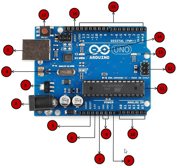
    1.电源USB

    Arduino 板可以通过使用计算机上的 USB 线供电。你需要做的是将USB 线连接到 USB 接口。

    2.电源(桶插座)

    Arduino 板可以通过将其连接到电源插口直接从交流电源供电。

    3.稳压器

    稳压器的功能是控制提供给 Arduino 板的电压,并稳定处理器和其他元件使用的直流电压。

    4.晶体振荡器

    它帮助
    帮助 Arduino 处理时间问题。Arduino 如何计算时间?答案是通过使用晶体振荡器。在 Arduino 晶体顶部打印的数字是16.000H9H。它告诉我们,频率是16,000,000赫兹或16MHz。

    5,17.Arduino 重置

    你可以重置你的Arduino 板,例如从一开始就启动你的程序。可以通过两种方式重置 UNO 板。首先,通过使用板上的复位按钮(17)。其次,你可以将外部复位按钮连接到标有RESET(5)的 Arduino 引脚。

    6,7,8,9.引脚(3.3,5,GND,Vin)

    • 3.3V(6) – 提供3.3输出电压
    • 5V(7) – 提供5输出电压
    • 使用3.3伏和5伏电压,与 Arduino 板一起使用的大多数组件可以正常工作。
    • GND(8)(接地) – Arduino上有几个GND引脚,其中任何一个都可用于将电路接地。
    • VVin(9) – 此引脚也可用于从外部电源(如交流主电源)为Arduino 板供电。

    10.模拟引脚

    Arduino UNO 板有六个模拟输入引脚,A0到A5。这些引脚可以从模拟传感器(如湿度传感器或温度传感器)读取信号,并将其转换为可由微处理器读取的数字值。

    11.微控制器

    每个 Arduino 板都有自己的微控制器(11)。你可以假设它作为板的大脑。Arduino 上的主IC(集成电路)与板对板略有不同。微控制器通常是 ATMEL 公司的。在从 Arduino IDE 加载新程序之前,你必须知道你的板上有什么IC。此信息位于IC顶部。

    12.ICSP引脚

    大多数情况下,ICSP(12)是一个AVR,一个由MOSI,MISO,SCK,RESET,VCC 和 GND 组成的 Arduino 的微型编程头。它通常被称为SPI(串行外设接口),可以被认为是输出的“扩展”。实际上,你是将输出设备从属到SPI总线的主机的。

    13.电源LED指示灯

    当你将 Arduino 插入电源时,此 LED 指示灯应亮起,表明你的电路板已正确通电。如果这个指示灯不亮,那么连接就出现了问题。

    14.TX 和 RX LED

    在你的板上,你会发现两个标签:TX(发送)和RX(接收)。它们出现在 Arduino UNO 板的两个地方。首先,在数字引脚0和1处,指示引脚负责串行通信。其次,TX 和 RX LED(13)。发送串行数据时,TX LED 以不同的速度闪烁。闪烁速度取决于板所使用的波特率。RX 在接收过程中闪烁。

    15.数字I/O

    Arduino UNO 板有14个数字I/O引脚(15)(其中6个提供 PWM(脉宽调制)输出),这些引脚可配置为数字输入引脚,用于读取逻辑值(0或1) ;或作为数字输出引脚来驱动不同的模块,如 LED,继电器等。标有“〜”的引脚可用于产生 PWM。

    16.AREF

    AREF代表模拟参考。它有时用于设置外部参考电压(0至5伏之间)作为模拟输入引脚的上限。

    如何安装 Arduino

    1、下载

    • 这个可以去官网:

      https://www.arduino.cc/en/Main/Software?setlang=cn

    在右边找到对应资源(这里以 Windows 为例),点击 Windows 安装包,即可开始下载

    注:免安装 ZIP 包也是可以的,不过可能会有问题。

    • 也可以去 Arduino 中文社区:

      http://www.arduino.cn/

    点击右面软件下载

    选择合适的下载即可。

    2、安装

    这个一路绿灯就可以了

    最后安装完成时会有如下弹窗:

    按照自己的需要安装就好。

    双击快捷方式即可开启。

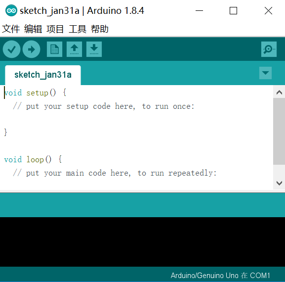
    之后打开工具,选择你所用的板子。再点击 serial port(串行端口),接入 Arduino 板,你会发现多了一个选项,那就是你的板子,选择它,设置就完成了。接下来就可以将程序上传到 Arduino 板里了。

    如何用 Arduino 写个简单的程序

    如果你已经试用过 Arduino IDE 并且没有问题了,那么你可以试试给你的板子上写点小东西玩了,首先先从最简单的 LED 灯开始吧,作为Arduino 的“Hello World”。

    我们以 Arduino Uno R3 为例

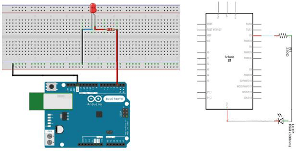
    你将需要:面包板×1  LED×1  330
    Ω 的电阻×1  一些跳线  以及你的Arduino Uno R3

    首先先接好电路,大概是这种感觉,要注意面包板中间部分的两列之间是不相通的,只有一列的五孔相通;而两侧部分则没有这种限制,只有特定的地方才不相通。

    然后打开你的 Arduino IDE,输入如下代码,a 是你所使用的引脚号码

    Void setup ( ) {
    
                pinMode(a,OUTPUT);
    
    }
    
    Void Loop ( ) {
    
                digitalWrite(a, HIGH);
    
                delay(1000);
    
                digitalWrite(a, LOW);
    
                delay(1000);
    
    }

    这段代码中用到了一些 Arduino 特有的函数:

    • pinMode(pin,mode)是在你使用 Arduino 的引脚前需要说明它的模式,INPUT,OUTPUT,或是 INPUT_PULLUP,不声明时默认为 INPUT。声明它为 OUTPUT 时,这个引脚可以提供电流,足以点亮 LED 或是运行传感器(千万别忘了串联一个电阻上去),但是试图运行需要高电流来工作的器件时可能会损坏引脚,虽然损坏一个暂时不是什么大问题,不过还是小心为好。
    • digitalWrite(pin,value)可以让你对引脚写入 HIGH 或 LOW,当引脚被声明为 OUTPUT 状态时,HIGH 将使输出电压提高,而 LOW 将会使输出电压变0。
    • delay(duration),延迟一段时间,duration以毫秒为单位。

    然后把这个代码上传到你的板子里,就能看到 LED 打开和关闭了。


    今日推荐英文原文:《Want to be a Web Developer? Learn Node.js not PHP》原文作者:Andrei Neagoie

    原文链接:https://hackernoon.com/want-to-be-a-web-developer-learn-node-js-not-php-dc298154fafd

    Want to be a Web Developer? Learn Node.js not PHP

    One of the most common questions I get asked by my students is “How come you teach Node.js and not PHP in your course?” Telling people “trust me, I work in the industry” simply isn’t enough. So, this is my reason for including Node.js in the course and why if you want to invest in your future as a developer, you should ditch PHP. Although I use these two as an example, in this article, I show you a framework for deciding on what tools, programming languages, frameworks, and libraries you should learn next throughout your developer career.

    With your limited time and resource as a developer, you have to make a decision on what to invest your time into to get the greatest return for this investment.

    Now, the question you should be asking yourself: What can I invest time and effort into learning that has the greatest net value on my future career as a developer in terms of knowledge, salary, and satisfaction?

    This doesn’t mean picking the easiest path. It means picking the tools that allow you to stay relevant and competitive for many years to come while also developing your skills to be a senior developer.

    In the Conclusion of this article, you will find all of the technologies I recommend in 2018 if you want to be a web developer using the same analysis done below. So you know, you can skip to the end if you’re impatient. Otherwise, grab a fair trade, organic, made with love, yerba mate tea and let’s go on a nerdy adventure.

    We are going to use two types of analysis in this post: Job Prospect Analysis and Technical Analysis. Here we go:

    source: https://vizteck.com/blog

    Node.js vs PHP — Job Prospect Analysis

    We will be using Stackoverflow developer survey and LinkedIn for this analysis. We will also only focus on technologies related to web development.

    Popularity:

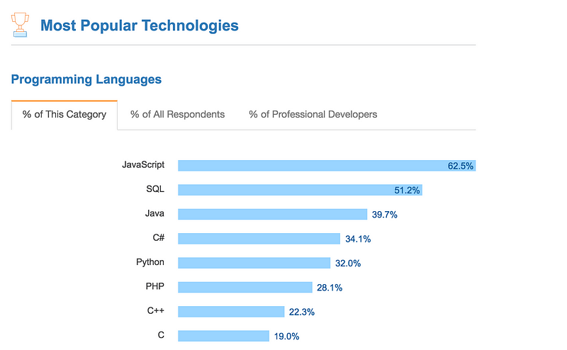
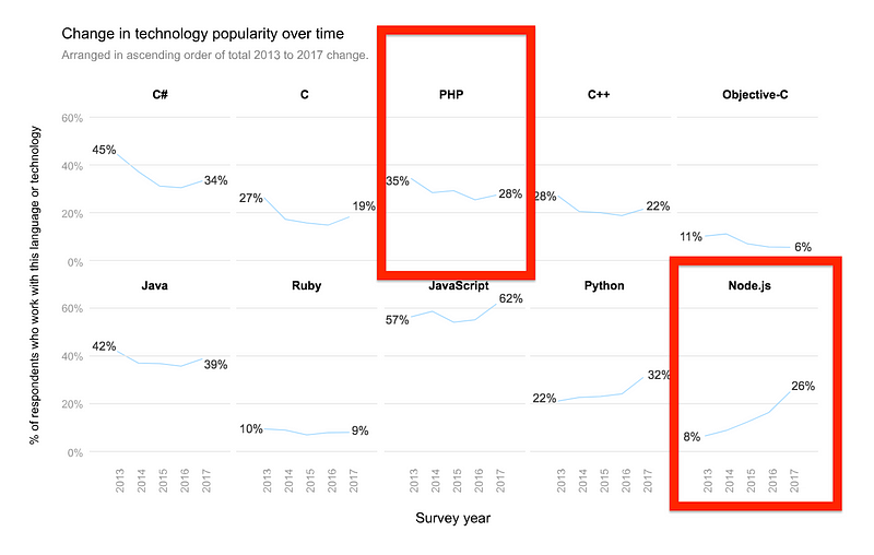
    For the fifth year in a row, JavaScript was the most commonly used programming language. The use of Python overtook PHP for the first time in five years. Where is Node.js in here? Node.js is a javascript runtime. In non technical speak: Node.js is a way to use Javascript like you can PHP on the server side. For now, think of Node.js as Javascript.

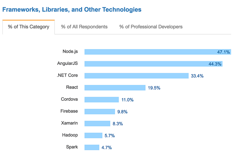
    As you can see, Node.js and Javascript rank at the top while PHP is significantly less popular.

    In the five years Stackoverflow has been collecting data in the Developer Survey, they have seen languages such as Javascript and Node.js grow in popularity, while the usage of languages like PHP has been shrinking:


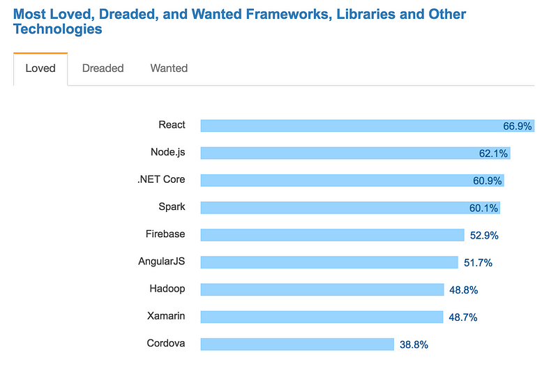
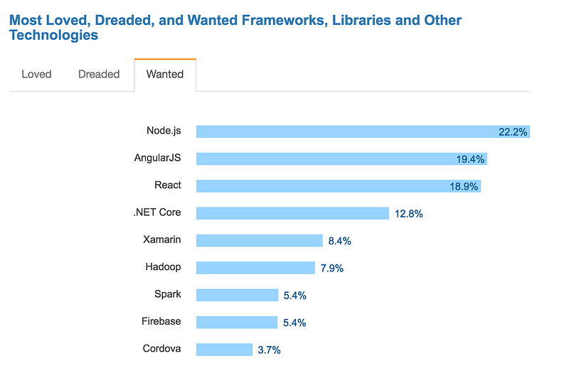
    React is the most loved among developers, however, Node.js is the most wanted and second most loved:


    Salaries and Opportunities:

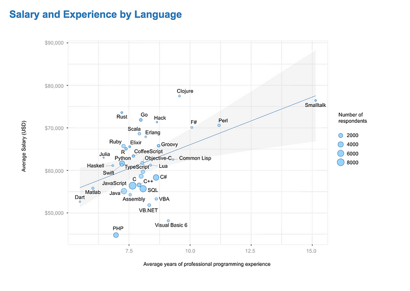
    Developers using languages listed below the blue line in the chart below, such as Go, Rust, and Clojure are being paid more given how much experience they have. Developers using languages below the blue line like PHP, however, are paid less even given years of experience. The size of the circles in this chart represents how many developers are using that language compared to the others. PHP significantly seems to be rewarding developers less and less with the number of years experience that they have.


    On LinkedIn Jobs, you can see the job posting worldwide for Node.js developers far outweighs PHP developers by almost 10,000. This is despite the fact that Node.js is a much younger technology compared to PHP, and the fact that PHP is used heavily with WordPress which powers 30% of all websites on the internet.


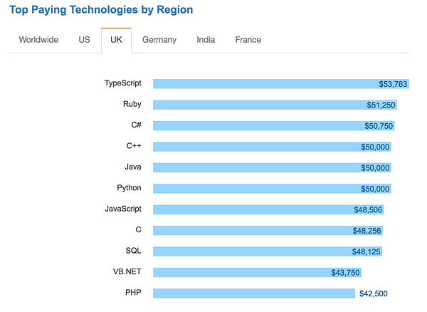
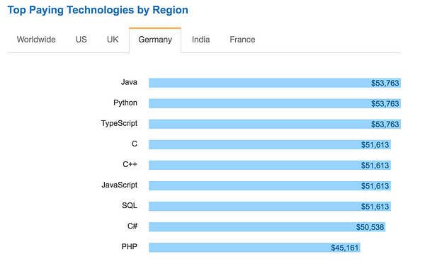
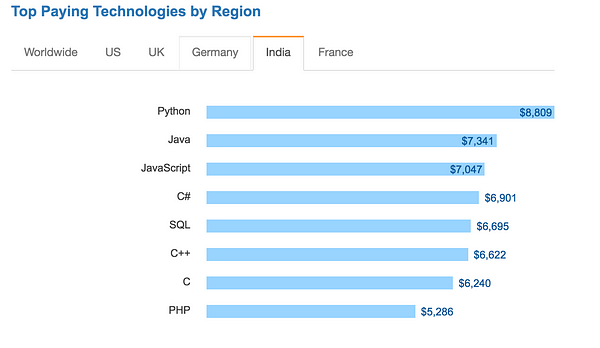
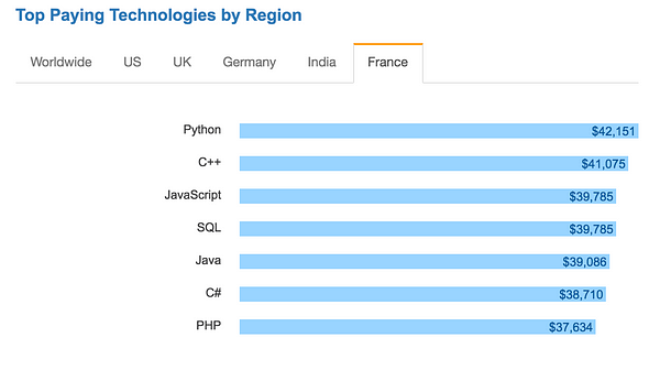
    Finally, you can see the average salary for technologies by Region (I didn’t include the Worldwide tab below because PHP didn’t even make it on there):

    Again, we are not bashing PHP here. We are just looking at the numbers to decide what to chose to learn. It is clearly ranking consistently below other technologies like Javascript and Node.js.

    UPDATE: Since releasing the post, stackoverflow came up with the result of the 2018 survey. The decline in PHP is growing.


    Verdict:

    PHP popularity is decreasing while the job market and popularity of Node.js is growing. Overall, PHP developers are paid significantly less than other developers and the trend seems to keep widening.


    Node.js vs PHP — Technical Analysis

    Let’s take a look at pros and cons of each technology.

    Node.js Pros:

    • Especially suitable for applications that require real time communication between client and server. Tools like socket.io make building things like chat applications really easy. This same features makes Node.js suitable for applications that process data from IoT devices (Internet of Things) and Single Page Applications (SPAs) which are very common now.
    • Native serialization and deserialization with JSON which works great with AJAX requests on the web.
    • Great for event driven applications that have non blocking Input/Output (I/O is the communication between an information processing system, such as a computer, and the outside world, possibly a human or another information processing systems like Databases)
    • You learn Javascript, you learn Node.js. You don’t need to learn another language like PHP. That means you can spend all your efforts learning Javascript really well and mastering it. You will be able to write both frontend and backend code with just one language.
    • Many popular client-side frameworks such as React, Vue, and Angular are written in JavaScript which is the main language of modern browsers. While using Node.js server-side, you have all the benefits of one scripting language across your application development stack. Having the same language both on the front and back end is excellent for maintainability: It makes the work between all team members easier for your application because both frontend and backend developers work with the same JavaScript data structures, functions, and language conventions.
    • The single-threaded event driven system is really fast when handling lots of requests at once from clients.
    • There are ever-growing 3rd party libraries and packages accessible through NPM for both client and server-side, as well as command-line tools for web development. Additionally, most of these are hosted on GitHub, where you can report an issue, or you can fork the code yourself to customize it.
    • It has become the standard environment in which to run Javascript related tools and other web developer related tools, including task runners, minifiers, linters, formatters, preprocessors, bundlers and analytics processors.
    • Natively supported on many new APIs and services like AWS Lambda.
    • We get all the performance gain of V8 which is the Google JavaScript interpreter that Node.js is built on top of. Since the Google’s engineering is constantly improving performance on V8, Node.js gets the benefit of this development for free.

    Node.js Cons:

    • NPM packages mentioned above can bloat your code, can be insecure, and it is hard to find which packages are good since there are so many options (Looking at downloads and GitHub stats is one way to fix this issue).
    • Huge number of ways to build servers using Node.js and npm packages. This makes it harder for new developers to pick up.
    • Not ideal for servers that are dependent on heavy CPU consuming code (i.e. heavy algorithms like image processing or sorting). Generally, anything that isn’t I/O can be thought of as CPU consuming code. Usually a multi-threaded server environment is a better option than Node.js in this case (Solution: if needed, you can hand CPU intensive parts of your code to a program written in C).
    • Node does not utilize all cores of an underlying system or machine. You have to write logic by yourself to use multi core processors. This can be achieved in many ways but it requires a bit of extra work (This becomes a pro when you are able to maximize CPU usage of the system).

    Node.js Verdict:

    Node.js is well suited for applications that have a lot of concurrent connections and each request only needs very few CPU cycles. This makes it extremely ideal for many of the applications currently on the internet like SPAs and real time applications.

    Using JavaScript’s built-in asynchronous processing, one can create highly scalable server-side code that maximize the usage of a single CPU and memory while being able to handle more concurrent requests than conventional multithreaded servers.

    Node.js comes with very few dependencies, rules and guidelines, which allow a developer to have the freedom and creativity in developing their applications the way they want to. Developers can select the best architecture, design patterns, modules and features for their project while getting all the benefit from the community through NPM.


    PHP Pros:

    • Strong and big community because of its age.
    • PHP has a powerful codebase that includes popular platforms for building websites (i.e. WordPress, Joomla, Drupal). CMS (Content Management Systems) such as WordPress, make it easy to deploy a blog or an e-commerce site in a matter of minutes and allow non-developers to customize them easily.
    • Easier to set up with non developer tools and preferred for individuals or small companies that don’t need to have knowledge of SSH and Linux servers. Numerous PHP applications (i.e. cPanel) are offered by basic hosting platforms which can be installed in one click.
    • Unlike other general purpose programming languages, PHP was designed specifically for the Web. PHP offers a great server side solution where there is no need to bother with JavaScript in the browser since all pages can be easily generated and rendered on the server. This is useful if you want to avoid shipping too much code on the client side. Node.js is able to do this as well, but the solution isn’t as simple.
    • PHP7 and HHVM (Supported by facebook) developments have improved on PHP performance.

    PHP Cons:

    • PHP is only used on the back end. This means you still need to learn Javascript if you want to work on the client side or be considered a full stack developer.
    • With PHP, heavy server-side rendering and numerous requests to the server to generate and render pages is not be a good option for Single Page Applications.
    • Each active client eats up one server process. Not ideal for apps with many client connections.
    • Native support for PHP on new APIs and services like AWS Lambda is limited compared to Node.js.
    • It follows the classical client-server model where every page request initiates the application, database connection, and HTML rendering. This makes PHP slower as you navigate through a website in comparison to Node.js application that runs permanently and needs only to initialize once. Because of this, Node.js is more suitable for the newer direction that the web is evolving into with HTML5, AJAX and WebSockets.

    PHP Verdict:

    PHP is simpler to learn with a big community around it. It is a good choice for a standardized solution such as blogs or news sites. It has the power of WordPress which is the most popular CMS (Content Management System) which allows you to create customizable blogs without too much coding. However, simpler in this case is not a good quality. The easier it is to learn a technology, the easier it is for someone to enter the field and increase the supply pool, and the lower you will have to charge for your services.


    Conclusion

    PHP was one of the top languages in the Web 1.0 era with the popularity of WordPress. Node.js was launched in 2009 and is technically not a language but a runtime environment for Javascript. It is the champion of a younger web development generation and is better suited for building event-based, data driven , I/O heavy applications that you encounter more in the Web 2.0 era.

    In particular, asynchronous and event-based architecture of Node.js makes it a great fit for real time applications such as messaging and collaborative apps in which many requests are happening concurrently and there is a lot of back and forth between the client and the server. Can’t live without WordPress? Well Node.js has it’s own CMS that is awesome called Keystone.js.

    There are always going to be tradeoffs. There is never going to be one technology that you can learn that will solve all problems and will make you immune to job obsolescence. The best we can do is to analyze our options and pick the one that will have best return on investment. Looking at the job prospect analysis and technical analysis above, we can see a clear winner.

    I pick Node.js.

    Although all technologies are great if used in their own specific way, we live in a world where information is so abundant that we have to limit the amount of topics we can focus on and deeply learn.

    In my course, I teach methodologies that are relevant today for a professional career in the field, and also the tools used by some of the biggest companies like Facebook, Netflix, Google and Amazon. If you want to be a full stack web developer in 2018, I recommend you learn:

    HTML5
    CSS3
    Javascript
    React.js
    Node.js + Express.js
    PostgreSQL

    and a few others…

    You can learn about them more by reading my article on learning to code in 2018 or checking out my online course that takes your from zero experience to having the skillset to get hired as a developer(only $10.99 with coupon code: MEDIUMNODE1723

    What are your thoughts?

    UPDATE: discussions around technologies should have opinions from both sides. I recommend you read through the comments. Keep in mind that there are always tradeoffs, and what tools you use in your profession is ultimately up to you. The best we can do is be informed about our choices and not follow blindly. Finally, be willing to consider opinions different than yours.


    每天推荐一个 GitHub 优质开源项目和一篇精选英文科技或编程文章原文,欢迎关注开源日报。交流QQ群:202790710;电报群 https://t.me/OpeningSourceOrg

  • 2018年4月1日:开源日报第24期

    1 4 月, 2018

    每天推荐一个 GitHub 优质开源项目和一篇精选英文科技或编程文章原文,欢迎关注开源日报。交流QQ群:202790710;电报群 https://t.me/OpeningSourceOrg


    今日推荐开源项目:《汇总资源宝库awesome》

    推荐理由:本项目提供了大量精选的阅读材料,旨在帮助后台开发者们能够借助项目中各个文献的思路做出一个具有延展性,可用性,稳定性的后台。这个概念虽然模糊,但是借由著名工程师(Martin Fowler,Robert C. Martin,Tom White等)和高质量资源(highscalability.com,infoq.com等)的诠释,相信大家能从中理解并学到有用的东西。

    项目将各类文献整理,涵盖各个方面。主要分为原则、可扩展性、稳定性、其他方面、会谈、图书七个板块。包括了异常处理,数据库策略等内容。

    什么是 awesome 项目

    这是 github 上一个有名的系列,项目名一般为 awesome-xxx ,这个系列一般是用来收集学习、工具、书籍类相关的项目,总之,这个系列一定能大大的满足您的收集癖.

    例如:

    awesome-python:https://github.com/vinta/awesome-python

    Python相关资源汇总

    Awesome-Linux-Software: https://github.com/LewisVo/Awesome-Linux-Software

    Linux上的好的软件及相关资源的汇总

    当然,还有一份大汇总列表,它的项目名就叫做awesome,链接:

    https://github.com/sindresorhus/awesome

    所以说,如果您不知道有什么资源可以用时,大可以在awesome 中查找,相信还是有很大的概率能得到您想要的东西的

    创建一个awesome 项目(列表)

    如果您有了与大家一起分享有趣或有价值的资源的想法,那不妨建立一个awesome 列表让更多的人一起参与进来,当然,请您务必参考awesome 提出的标准,链接:

    https://github.com/sindresorhus/awesome/blob/master/create-list.md


    作者:Benny Nguyen

    新加坡软件工程师(分布式系统&大数据)

    新加坡人

    在越南国立大学获得本科学位,在新加坡过哦立大学获得计算机硕士学位

    技能专长如算法,java,c++,c#等多达25项


    今日推荐英文原文:《Ten Machine Learning Algorithms You Should Know to Become a Data Scientist》作者:Shashank Gupta

    原文链接:https://towardsdatascience.com/ten-machine-learning-algorithms-you-should-know-to-become-a-data-scientist-8dc93d8ca52e

    推荐理由:机器学习热度持续不减,一方面有市场炒作,一方面其本身的魅力令让难当,尤其是加持数据之美,海量的数据加上机器学习算法真的可以碰撞出很赞的火花,这篇文章就给大家介绍了10个机器学习算法,如果你想成为一个数据科学家?这篇文章正好。


    Ten Machine Learning Algorithms You Should Know to Become a Data Scientist

    Machine Learning Practitioners have different personalities. While some of them are “I am an expert in X and X can train on any type of data”, where X = some algorithm, some others are “Right tool for the right job people”. A lot of them also subscribe to “Jack of all trades. Master of one” strategy, where they have one area of deep expertise and know slightly about different fields of Machine Learning. That said, no one can deny the fact that as practicing Data Scientists, we will have to know basics of some common machine learning algorithms, which would help us engage with a new-domain problem we come across. This is a whirlwind tour of common machine learning algorithms and quick resources about them which can help you get started on them.

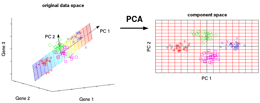
    1. Principal Component Analysis(PCA)/SVD

    PCA is an unsupervised method to understand global properties of a dataset consisting of vectors. Covariance Matrix of data points is analyzed here to understand what dimensions(mostly)/ data points (sometimes) are more important (ie have high variance amongst themselves, but low covariance with others). One way to think of top PCs of a matrix is to think of its eigenvectors with highest eigenvalues. SVD is essentially a way to calculate ordered components too, but you don’t need to get the covariance matrix of points to get it.

    This Algorithm helps one fight curse of dimensionality by getting datapoints with reduced dimensions.

    Libraries:

    https://docs.scipy.org/doc/scipy/reference/generated/scipy.linalg.svd.html

    http://scikit-learn.org/stable/modules/generated/sklearn.decomposition.PCA.html

    Introductory Tutorial:

    https://arxiv.org/pdf/1404.1100.pdf

    2a. Least Squares and Polynomial Fitting

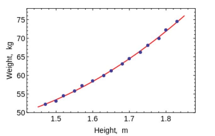
    Remember your Numerical Analysis code in college, where you used to fit lines and curves to points to get an equation. You can use them to fit curves in Machine Learning for very small datasets with low dimensions. (For large data or datasets with many dimensions, you might just end up terribly overfitting, so don’t bother). OLS has a closed form solution, so you don’t need to use complex optimization techniques.

    As is obvious, use this algorithm to fit simple curves / regression

    Libraries:

    https://docs.scipy.org/doc/numpy/reference/generated/numpy.linalg.lstsq.htmlhttps://docs.scipy.org/doc/numpy-1.10.0/reference/generated/numpy.polyfit.html

    Introductory Tutorial:

    https://lagunita.stanford.edu/c4x/HumanitiesScience/StatLearning/asset/linear_regression.pdf

    2b. Constrained Linear Regression

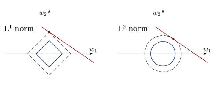
    Least Squares can get confused with outliers, spurious fields and noise in data. We thus need constraints to decrease the variance of the line we fit on a dataset. The right method to do it is to fit a linear regression model which will ensure that the weights do not misbehave. Models can have L1 norm (LASSO) or L2 (Ridge Regression) or both (elastic regression). Mean Squared Loss is optimized.

    Use these algorithms to fit regression lines with constraints, avoiding overfitting and masking noise dimensions from model.

    Libraries:

    http://scikit-learn.org/stable/modules/linear_model.html

    Introductory Tutorial(s):

    https://www.youtube.com/watch?v=5asL5Eq2x0A

    https://www.youtube.com/watch?v=jbwSCwoT51M

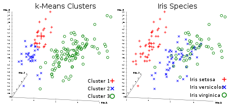
    3. K means Clustering

    Everyone’s favorite unsupervised clustering algorithm. Given a set of data points in form of vectors, we can make clusters of points based on distances between them. It’s an Expectation Maximization algorithm that iteratively moves the centers of clusters and then clubs points with each cluster centers. The input the algorithm has taken is the number of clusters which are to be generated and the number of iterations in which it will try to converge clusters.

    As is obvious from the name, you can use this algorithm to create K clusters in dataset

    Library:

    http://scikit-learn.org/stable/modules/generated/sklearn.cluster.KMeans.html

    Introductory Tutorial(s):

    https://www.youtube.com/watch?v=hDmNF9JG3lo

    https://www.datascience.com/blog/k-means-clustering

    4. Logistic Regression

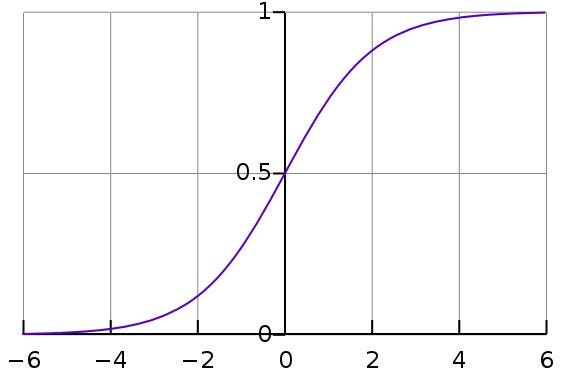
    Logistic Regression is constrained Linear Regression with a nonlinearity (sigmoid function is used mostly or you can use tanh too) application after weights are applied, hence restricting the outputs close to +/- classes (which is 1 and 0 in case of sigmoid). Cross-Entropy Loss functions are optimized using Gradient Descent. A note to beginners: Logistic Regression is used for classification, not regression. You can also think of Logistic regression as a one layered Neural Network. Logistic Regression is trained using optimization methods like Gradient Descent or L-BFGS. NLP people will often use it with the name of Maximum Entropy Classifier.

    This is what a Sigmoid looks like:

    Use LR to train simple, but very robust classifiers.

    Library:

    http://scikit-learn.org/stable/modules/generated/sklearn.linear_model.LogisticRegression.html

    Introductory Tutorial(s):

    https://www.youtube.com/watch?v=-la3q9d7AKQ

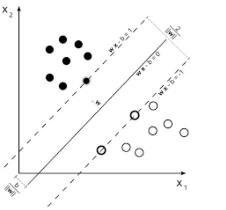
    5. SVM (Support Vector Machines)

    SVMs are linear models like Linear/ Logistic Regression, the difference is that they have different margin-based loss function (The derivation of Support Vectors is one of the most beautiful mathematical results I have seen along with eigenvalue calculation). You can optimize the loss function using optimization methods like L-BFGS or even SGD.

    Another innovation in SVMs is the usage of kernels on data to feature engineer. If you have good domain insight, you can replace the good-old RBF kernel with smarter ones and profit.

    One unique thing that SVMs can do is learn one class classifiers.

    SVMs can used to Train a classifier (even regressors)

    Library:

    http://scikit-learn.org/stable/modules/generated/sklearn.svm.SVC.html

    Introductory Tutorial(s):

    https://www.youtube.com/watch?v=eHsErlPJWUU

    Note: SGD based training of both Logistic Regression and SVMs are found in SKLearn’s http://scikit-learn.org/stable/modules/generated/sklearn.linear_model.SGDClassifier.html , which I often use as it lets me check both LR and SVM with a common interface. You can also train it on >RAM sized datasets using mini batches.

    6. Feedforward Neural Networks

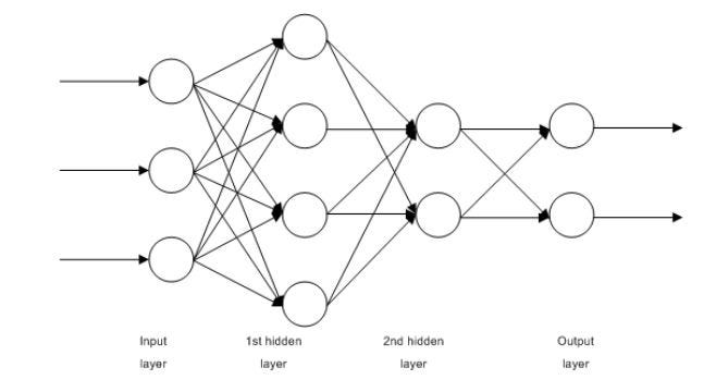
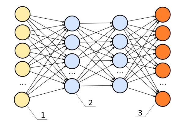
    These are basically multilayered Logistic Regression classifiers. Many layers of weights separated by non-linearities (sigmoid, tanh, relu + softmax and the cool new selu). Another popular name for them is Multi-Layered Perceptrons. FFNNs can be used for classification and unsupervised feature learning as autoencoders.

    Multi-Layered perceptron
    FFNN as an autoencoder

    FFNNs can be used to train a classifier or extract features as autoencoders

    Libraries:

    http://scikit-learn.org/stable/modules/generated/sklearn.neural_network.MLPClassifier.html#sklearn.neural_network.MLPClassifier

    http://scikit-learn.org/stable/modules/generated/sklearn.neural_network.MLPRegressor.html

    https://github.com/keras-team/keras/blob/master/examples/reuters_mlp_relu_vs_selu.py

    Introductory Tutorial(s):

    http://www.deeplearningbook.org/contents/mlp.html

    http://www.deeplearningbook.org/contents/autoencoders.html

    http://www.deeplearningbook.org/contents/representation.html

    7. Convolutional Neural Networks (Convnets)

    Almost any state of the art Vision based Machine Learning result in the world today has been achieved using Convolutional Neural Networks. They can be used for Image classification, Object Detection or even segmentation of images. Invented by Yann Lecun in late 80s-early 90s, Convnets feature convolutional layers which act as hierarchical feature extractors. You can use them in text too (and even graphs).

    Use convnets for state of the art image and text classification, object detection, image segmentation.

    Libraries:

    https://developer.nvidia.com/digits

    https://github.com/kuangliu/torchcv

    https://github.com/chainer/chainercv

    https://keras.io/applications/

    Introductory Tutorial(s):

    http://cs231n.github.io/

    https://adeshpande3.github.io/A-Beginner%27s-Guide-To-Understanding-Convolutional-Neural-Networks/

    8. Recurrent Neural Networks (RNNs):

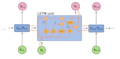
    RNNs model sequences by applying the same set of weights recursively on the aggregator state at a time t and input at a time t (Given a sequence has inputs at times 0..t..T, and have a hidden state at each time t which is output from t-1 step of RNN). Pure RNNs are rarely used now but its counterparts like LSTMs and GRUs are state of the art in most sequence modeling tasks.

    RNN (If here is a densely connected unit and a nonlinearity, nowadays f is generally LSTMs or GRUs ). LSTM unit which is used instead of a plain dense layer in a pure RNN.

    Use RNNs for any sequence modelling task specially text classification, machine translation, language modelling

    Library:

    https://github.com/tensorflow/models (Many cool NLP research papers from Google are here)

    https://github.com/wabyking/TextClassificationBenchmark

    http://opennmt.net/

    Introductory Tutorial(s):

    http://cs224d.stanford.edu/

    http://www.wildml.com/category/neural-networks/recurrent-neural-networks/

    http://colah.github.io/posts/2015-08-Understanding-LSTMs/

    9. Conditional Random Fields (CRFs)

    CRFs are probably the most frequently used models from the family of Probabilitic Graphical Models (PGMs). They are used for sequence modeling like RNNs and can be used in combination with RNNs too. Before Neural Machine Translation systems came in CRFs were the state of the art and in many sequence tagging tasks with small datasets, they will still learn better than RNNs which require a larger amount of data to generalize. They can also be used in other structured prediction tasks like Image Segmentation etc. CRF models each element of the sequence (say a sentence) such that neighbors affect a label of a component in a sequence instead of all labels being independent of each other.

    Use CRFs to tag sequences (in Text, Image, Time Series, DNA etc.)

    Library:

    https://sklearn-crfsuite.readthedocs.io/en/latest/

    Introductory Tutorial(s):

    http://blog.echen.me/2012/01/03/introduction-to-conditional-random-fields/

    7 part lecture series by Hugo Larochelle on Youtube: https://www.youtube.com/watch?v=GF3iSJkgPbA

    10. Decision Trees

    Let’s say I am given an Excel sheet with data about various fruits and I have to tell which look like Apples. What I will do is ask a question “Which fruits are red and round ?” and divide all fruits which answer yes and no to the question. Now, All Red and Round fruits might not be apples and all apples won’t be red and round. So I will ask a question “Which fruits have red or yellow color hints on them? ” on red and round fruits and will ask “Which fruits are green and round ?” on not red and round fruits. Based on these questions I can tell with considerable accuracy which are apples. This cascade of questions is what a decision tree is. However, this is a decision tree based on my intuition. Intuition cannot work on high dimensional and complex data. We have to come up with the cascade of questions automatically by looking at tagged data. That is what Machine Learning based decision trees do. Earlier versions like CART trees were once used for simple data, but with bigger and larger dataset, the bias-variance tradeoff needs to solved with better algorithms. The two common decision trees algorithms used nowadays are Random Forests (which build different classifiers on a random subset of attributes and combine them for output) and Boosting Trees (which train a cascade of trees one on top of others, correcting the mistakes of ones below them).
    Decision Trees can be used to classify datapoints (and even regression)

    Libraries

    http://scikit-learn.org/stable/modules/generated/sklearn.ensemble.RandomForestClassifier.html

    http://scikit-learn.org/stable/modules/generated/sklearn.ensemble.GradientBoostingClassifier.html

    http://xgboost.readthedocs.io/en/latest/

    https://catboost.yandex/

    Introductory Tutorial:

    http://xgboost.readthedocs.io/en/latest/model.html

    https://arxiv.org/abs/1511.05741

    https://arxiv.org/abs/1407.7502

    http://education.parrotprediction.teachable.com/p/practical-xgboost-in-python

    TD Algorithms (Good To Have)

    If you are still wondering how can any of the above methods solve tasks like defeating Go world champion like DeepMind did, they cannot. All the 10 type of algorithms we talked about before this was Pattern Recognition, not strategy learners. To learn strategy to solve a multi-step problem like winning a game of chess or playing Atari console, we need to let an agent-free in the world and learn from the rewards/penalties it faces. This type of Machine Learning is called Reinforcement Learning. A lot (not all) of recent successes in the field is a result of combining perception abilities of a convent or a LSTM to a set of algorithms called Temporal Difference Learning. These include Q-Learning, SARSA and some other variants. These algorithms are a smart play on Bellman’s equations to get a loss function that can be trained with rewards an agent gets from the environment.

    These algorithms are used to automatically play games mostly :D, also other applications in language generation and object detection.

    Libraries:

    https://github.com/keras-rl/keras-rl

    https://github.com/tensorflow/minigo

    Introductory Tutorial(s):

    Grab the free Sutton and Barto book: https://web2.qatar.cmu.edu/~gdicaro/15381/additional/SuttonBarto-RL-5Nov17.pdf

    Watch David Silver course: https://www.youtube.com/watch?v=2pWv7GOvuf0

    These are the 10 machine learning algorithms which you can learn to become a data scientist.

    You can also read about machine learning libraries here.

    We hope you liked the article. Please Sign Up for a free ParallelDots account to start your AI journey. You can also check demo’s of our APIs here.


    每天推荐一个 GitHub 优质开源项目和一篇精选英文科技或编程文章原文,欢迎关注开源日报。交流QQ群:202790710;电报群 https://t.me/OpeningSourceOrg

←上一页
1 … 253 254 255 256 257 … 262
下一页→

Proudly powered by WordPress