2018年5月22日：开源日报第75期

22 5 月, 2018
每天推荐一个 GitHub 优质开源项目和一篇精选英文科技或编程文章原文，欢迎关注开源日报。交流QQ群：202790710；微博：https://weibo.com/openingsource；电报群 https://t.me/OpeningSourceOrg

今日推荐开源项目：《图形界面开发库 LCUI》

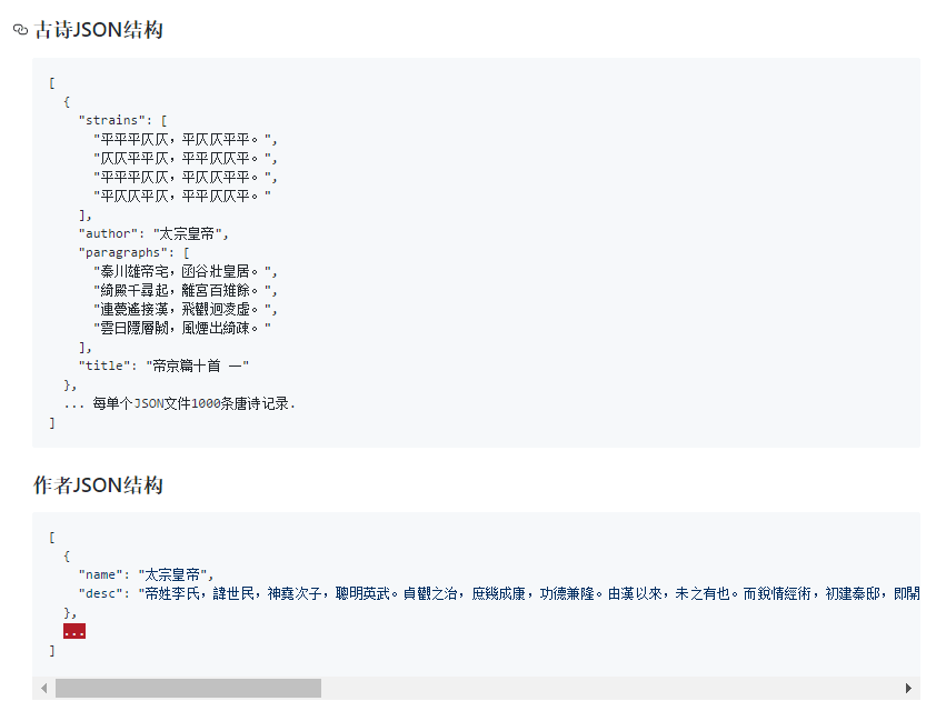
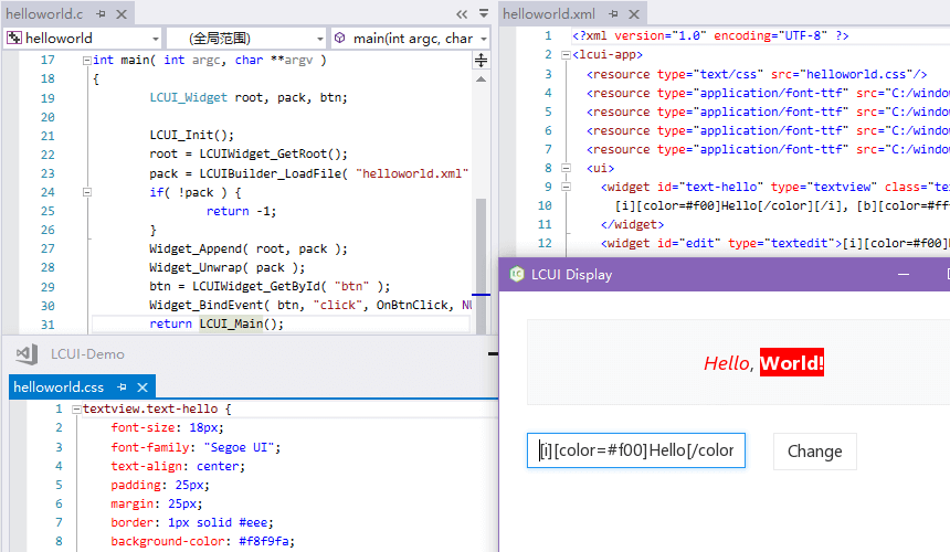
推荐理由：LCUI 是一种自由和开放源代码的图形界面开发库，主要使用 C 语言编写，支持使用 CSS 和 XML 描述界面结构和样式，可用于构建简单的桌面应用程序。

主要特性
- C 语言编写
- 跨平台
- XML 解析
- CSS 解析
- 类 HTML 布局
- 界面缩放
- 文本绘制
- 字体管理
- 图片处理
- 触控
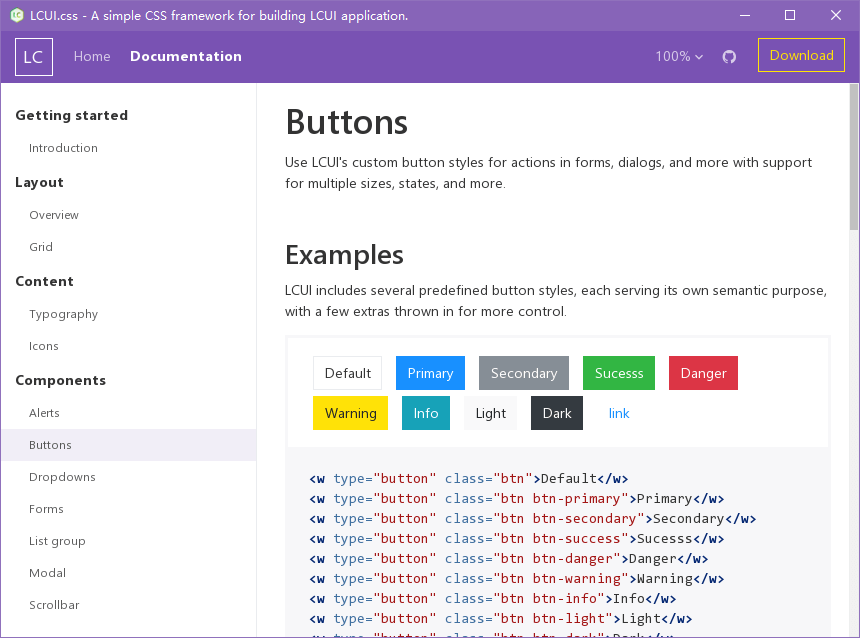
luci.css

今日推荐英文原文：《Linux vs. Unix: What’s the difference?》作者： Phil Estes

原文链接：https://opensource.com/article/18/5/differences-between-linux-and-unix

推荐理由：Linux 和 Unix 有什么不同呢？

Linux vs. Unix: What’s the difference?

f you are a software developer in your 20s or 30s, you’ve grown up in a world dominated by Linux. It has been a significant player in the data center for decades, and while it’s hard to find definitive operating system market share reports, Linux’s share of data center operating systems could be as high as 70%, with Windows variants carrying nearly all the remaining percentage. Developers using any major public cloud can expect the target system will run Linux. Evidence that Linux is everywhere has grown in recent years when you add in Android and Linux-based embedded systems in smartphones, TVs, automobiles, and many other devices.

Even so, most software developers, even those who have grown up during this venerable “Linux revolution” have at least heard of Unix. It sounds similar to Linux, and you’ve probably heard people use these terms interchangeably. Or maybe you’ve heard Linux called a “Unix-like” operating system.

So, what is this Unix? The caricatures speak of wizard-like “graybeards” sitting behind glowing green screens, writing C code and shell scripts, powered by old-fashioned, drip-brewed coffee. But Unix has a much richer history beyond those bearded C programmers from the 1970s. While articles detailing the history of Unix and “Unix vs. Linux” comparisons abound, this article will offer a high-level background and a list of major differences between these complementary worlds.

Unix’s beginnings

The history of Unix begins at AT&T Bell Labs in the late 1960s with a small team of programmers looking to write a multi-tasking, multi-user operating system for the PDP-7. Two of the most notable members of this team at the Bell Labs research facility were Ken Thompson and Dennis Ritchie. While many of Unix’s concepts were derivative of its predecessor (Multics), the Unix team’s decision early in the 1970s to rewrite this small operating system in the C language is what separated Unix from all others. At the time, operating systems were rarely, if ever, portable. Instead, by nature of their design and low-level source language, operating systems were tightly linked to the hardware platform for which they had been authored. By refactoring Unix on the C programming language, Unix could now be ported to many hardware architectures.

In addition to this new portability, which allowed Unix to quickly expand beyond Bell Labs to other research, academic, and even commercial uses, several key of the operating system’s design tenets were attractive to users and programmers. For one, Ken Thompson’s Unix philosophy became a powerful model of modular software design and computing. The Unix philosophy recommended utilizing small, purpose-built programs in combination to do complex overall tasks. Since Unix was designed around files and pipes, this model of “piping” inputs and outputs of programs together into a linear set of operations on the input is still in vogue today. In fact, the current cloud functions-as-a-service (FaaS)/serverless computing model owes much of its heritage to the Unix philosophy.

Rapid growth and competition

Through the late 1970s and 80s, Unix became the root of a family tree that expanded across research, academia, and a growing commercial Unix operating system business. Unix was not open source software, and the Unix source code was licensable via agreements with its owner, AT&T. The first known software license was sold to the University of Illinois in 1975.

Unix grew quickly in academia, with Berkeley becoming a significant center of activity, given Ken Thompson’s sabbatical there in the ’70s. With all the activity around Unix at Berkeley, a new delivery of Unix software was born: the Berkeley Software Distribution, or BSD. Initially, BSD was not an alternative to AT&T’s Unix, but an add-on with additional software and capabilities. By the time 2BSD (the Second Berkeley Software Distribution) arrived in 1979, Bill Joy, a Berkeley grad student, had added now-famous programs such as vi and the C shell (/bin/csh).

In addition to BSD, which became one of the most popular branches of the Unix family, Unix’s commercial offerings exploded through the 1980s and into the ’90s with names like HP-UX, IBM’s AIX, Sun’s Solaris, Sequent, and Xenix. As the branches grew from the original root, the “Unix wars” began, and standardization became a new focus for the community. The POSIX standard was born in 1988, as well as other standardization follow-ons via The Open Group into the 1990s.

Around this time AT&T and Sun released System V Release 4 (SVR4), which was adopted by many commercial vendors. Separately, the BSD family of operating systems had grown over the years, leading to some open source variations that were released under the now-familiar BSD license. This included FreeBSD, OpenBSD, and NetBSD, each with a slightly different target market in the Unix server industry. These Unix variants continue to have some usage today, although many have seen their server market share dwindle into the single digits (or lower). BSD may have the largest install base of any modern Unix system today. Also, every Apple Mac hardware unit shipped in recent history can be claimed by BSD, as its OS X (now macOS) operating system is a BSD-derivative.

While the full history of Unix and its academic and commercial variants could take many more pages, for the sake of our article focus, let’s move on to the rise of Linux.

Enter Linux

What we call the Linux operating system today is really the combination of two efforts from the early 1990s. Richard Stallman was looking to create a truly free and open source alternative to the proprietary Unix system. He was working on the utilities and programs under the name GNU, a recursive algorithm meaning “GNU’s not Unix!” Although there was a kernel project underway, it turned out to be difficult going, and without a kernel, the free and open source operating system dream could not be realized. It was Linus Torvald’s work—producing a working and viable kernel that he called Linux—that brought the complete operating system to life. Given that Linus was using several GNU tools (e.g., the GNU Compiler Collection, or GCC), the marriage of the GNU tools and the Linux kernel was a perfect match.

Linux distributions came to life with the components of GNU, the Linux kernel, MIT’s X-Windows GUI, and other BSD components that could be used under the open source BSD license. The early popularity of distributions like Slackware and then Red Hat gave the “common PC user” of the 1990s access to the Linux operating system and, with it, many of the proprietary Unix system capabilities and utilities they used in their work or academic lives.

Because of the free and open source standing of all the Linux components, anyone could create a Linux distribution with a bit of effort, and soon the total number of distros reached into the hundreds. Today, distrowatch.com lists 312 unique Linux distributions available in some form. Of course, many developers utilize Linux either via cloud providers or by using popular free distributions like Fedora, Canonical’s Ubuntu, Debian, Arch Linux, Gentoo, and many other variants. Commercial Linux offerings, which provide support on top of the free and open source components, became viable as many enterprises, including IBM, migrated from proprietary Unix to offering middleware and software solutions atop Linux. Red Hat built a model of commercial support around Red Hat Enterprise Linux, as did German provider SUSE with SUSE Linux Enterprise Server (SLES).

Comparing Unix and Linux

So far, we’ve looked at the history of Unix and the rise of Linux and the GNU/Free Software Foundation underpinnings of a free and open source alternative to Unix. Let’s examine the differences between these two operating systems that share much of the same heritage and many of the same goals.

From a user experience perspective, not very much is different! Much of the attraction of Linux was the operating system’s availability across many hardware architectures (including the modern PC) and ability to use tools familiar to Unix system administrators and users.

Because of POSIX standards and compliance, software written on Unix could be compiled for a Linux operating system with a usually limited amount of porting effort. Shell scripts could be used directly on Linux in many cases. While some tools had slightly different flag/command-line options between Unix and Linux, many operated the same on both.

One side note is that the popularity of the macOS hardware and operating system as a platform for development that mainly targets Linux may be attributed to the BSD-like macOS operating system. Many tools and scripts meant for a Linux system work easily within the macOS terminal. Many open source software components available on Linux are easily available through tools like Homebrew.

The remaining differences between Linux and Unix are mainly related to the licensing model: open source vs. proprietary, licensed software. Also, the lack of a common kernel within Unix distributions has implications for software and hardware vendors. For Linux, a vendor can create a device driver for a specific hardware device and expect that, within reason, it will operate across most distributions. Because of the commercial and academic branches of the Unix tree, a vendor might have to write different drivers for variants of Unix and have licensing and other concerns related to access to an SDK or a distribution model for the software as a binary device driver across many Unix variants.

As both communities have matured over the past decade, many of the advancements in Linux have been adopted in the Unix world. Many GNU utilities were made available as add-ons for Unix systems where developers wanted features from GNU programs that aren’t part of Unix. For example, IBM’s AIX offered an AIX Toolbox for Linux Applications with hundreds of GNU software packages (like Bash, GCC, OpenLDAP, and many others) that could be added to an AIX installation to ease the transition between Linux and Unix-based AIX systems.

Proprietary Unix is still alive and well and, with many major vendors promising support for their current releases well into the 2020s, it goes without saying that Unix will be around for the foreseeable future. Also, the BSD branch of the Unix tree is open source, and NetBSD, OpenBSD, and FreeBSD all have strong user bases and open source communities that may not be as visible or active as Linux, but are holding their own in recent server share reports, with well above the proprietary Unix numbers in areas like web serving.

Where Linux has shown a significant advantage over proprietary Unix is in its availability across a vast number of hardware platforms and devices. The Raspberry Pi, popular with hobbyists and enthusiasts, is Linux-driven and has opened the door for an entire spectrum of IoT devices running Linux. We’ve already mentioned Android devices, autos (with Automotive Grade Linux), and smart TVs, where Linux has large market share. Every cloud provider on the planet offers virtual servers running Linux, and many of today’s most popular cloud-native stacks are Linux-based, whether you’re talking about container runtimes or Kubernetes or many of the serverless platforms that are gaining popularity.

One of the most revealing representations of Linux’s ascendancy is Microsoft’s transformation in recent years. If you told software developers a decade ago that the Windows operating system would “run Linux” in 2016, most of them would have laughed hysterically. But the existence and popularity of the Windows Subsystem for Linux (WSL), as well as more recently announced capabilities like the Windows port of Docker, including LCOW (Linux containers on Windows) support, are evidence of the impact that Linux has had—and clearly will continue to have—across the software world.

每天推荐一个 GitHub 优质开源项目和一篇精选英文科技或编程文章原文，欢迎关注开源日报。交流QQ群：202790710；微博：https://weibo.com/openingsource；电报群 https://t.me/OpeningSourceOrg
2018年5月21日：开源日报第74期

20 5 月, 2018
每天推荐一个 GitHub 优质开源项目和一篇精选英文科技或编程文章原文，欢迎关注开源日报。交流QQ群：202790710；微博：https://weibo.com/openingsource；电报群 https://t.me/OpeningSourceOrg

今日推荐开源项目：《超级备忘录——Awesome-Cheatsheets》

推荐理由：你可以把Awesome-Cheatsheets看作是一个备忘录，其实它的作用与备忘录很相似，但它又不止是一个备忘录，姑且叫“超级备忘录”好了！

这是一个存储了现在流行的编程语言，框架和开发工具的使用技巧和知识的地方，记录的许多人在使用一些语言，框架和工具的途中积累下来的知识于技巧，比如JavaScript，Bash, Node.js等。

Awesome-Cheatsheets就是这样一个工具。我们在学习一门新技巧，新语言时，许多人都会选择做一个Cheatsheets，随着时间的积累，我们积累的东西也会越来越多，Awesome-Cheatshoots系统的存储记录了这些零碎的知识。使用它将会是一个不错的体验。

Awesome-Cheatsheets现在还在继续完善中，不断收集在学习各种语言，框架，工具的知识，我想它一定会满足我们对知识的需求。

今日推荐英文原文：《Introducing Git protocol version 2》作者：Brandon Williams, Git Core Team

原文链接：https://opensource.googleblog.com/2018/05/introducing-git-protocol-version-2.html

推荐理由：Google 正式在其官方 Blog 宣布 Git protocal version 2，这个版本最主要的变化是客户端与服务器端一些 clone、fetch、push等一些操作的协议。

Introducing Git protocol version 2

Today we announce Git protocol version 2, a major update of Git’s wire protocol (how clones, fetches and pushes are communicated between clients and servers). This update removes one of the most inefficient parts of the Git protocol and fixes an extensibility bottleneck, unblocking the path to more wire protocol improvements in the future.

The protocol version 2 spec can be found here. The main improvements are:
- Server-side filtering of references
- Easy extensibility for new features like ref-in-want and fetching and pushing symrefs
- Simplified client handling of the http transport
The main motivation for the new protocol was to enable server side filtering of references (branches and tags). Prior to protocol v2, servers responded to all fetch commands with an initial reference advertisement, listing all references in the repository. This complete listing is sent even when a client only cares about updating a single branch, e.g.: `git fetch origin master`. For repositories that contain 100s of thousands of references (the Chromium repository has over 500k branches and tags) the server could end up sending 10s of megabytes of data that get ignored. This typically dominates both time and bandwidth during a fetch, especially when you are updating a branch that’s only a few commits behind the remote, or even when you are only checking if you are up-to-date, resulting in a no-op fetch.

We recently rolled out support for protocol version 2 at Google and have seen a performance improvement of 3x for no-op fetches of a single branch on repositories containing 500k references. Protocol v2 has also enabled a reduction of 8x of the overhead bytes (non-packfile) sent from googlesource.com servers. A majority of this improvement is due to filtering references advertised by the server to the refs the client has expressed interest in.

Getting over the hurdles

The Git project has tried on a number of occasions over the years to either limit the initial ref advertisement or move to a new protocol altogether but continued to run into two problems: (1) the initial request is rigid and does not include a field that could be used to request that new servers modify their response without breaking compatibility with existing servers and (2) error handling is not well enough defined to allow safely using a new protocol that existing servers do not understand with a quick fallback to the old protocol. To migrate to a new protocol version, we needed to find a side channel which existing servers would ignore but could be used to safely communicate with newer servers.

There are three main transports that are used to speak Git’s wire-protocol (git://, ssh://, and https://), and the side channel that we use to request v2 needs to communicate in such a way that an older server would ignore any additional data sent and not crash. The http transport was the easiest as we can simply include an additional http header in the request (“Git-Protocol: version=2”). The ssh transport is a bit more difficult as it requires sending an environment variable (“GIT_PROTOCOL=version=2”) to be set on the remote end. This is more challenging because it requires server administrators to configure sshd to accept the new environment variable on their server. The most difficult transport is the anonymous Git transport (git://).

Initial requests made to a server using the anonymous Git transport are made in the form of a single packet-line which includes the requested service (git-upload-pack for fetches and git-receive-pack for pushes), and the repository followed by a NUL byte. Later virtualization support was added and a hostname parameter could be tacked on and terminated by a NUL byte: `0033git-upload-pack /project.git\0host=myserver.com\0`. Ideally we’d be able to add a new parameter to be used to request v2 by adding it in the same manner as the hostname was added: `003dgit-upload-pack /project.git\0host=myserver.com\0version=2\0`. Unfortunately due to a bug introduced in 2006 we aren’t able to place any extra arguments (separated by NULs) other than the host because otherwise the parsing of those arguments would enter an infinite loop. When this bug was fixed in 2009, a check was put in place to disallow extra arguments so that new clients wouldn’t trigger this bug in older servers.

Fortunately, that check doesn’t notice if we send additional request arguments hidden behind a second NUL byte, which was pointed out back in 2009. This allows requests structured like: `003egit-upload-pack /project.git\0host=myserver.com\0\0version=2\0`. By placing version information behind a second NUL byte we can skirt around both the infinite loop bug and the explicit disallowal of extra arguments besides hostname. Only newer servers will know to look for additional information hidden behind two NUL bytes and older servers won’t croak.

Now, in every case, a client can issue a request to use v2, using a transport-specific side channel, and v2 servers can respond using the new protocol while older servers will ignore the side channel and just respond with a ref advertisement.

Try it for yourself

To try out protocol version 2 for yourself you’ll need an up to date version of Git (support for v2 was recently merged to Git’s master branch and is expected to be part of Git 2.18) and a v2 enabled server (repositories on googlesource.com and Cloud Source Repositories are v2 enabled). If you enable tracing and run the `ls-remote` command querying for a single branch, you can see the server sends a much smaller set of references when using protocol version 2:

# Using the original wire protocol

GIT_TRACE_PACKET=1 git -c protocol.version=0 ls-remote https://chromium.googlesource.com/chromium/src.git master

# Using protocol version 2

GIT_TRACE_PACKET=1 git -c protocol.version=2 ls-remote https://chromium.googlesource.com/chromium/src.git master

每天推荐一个 GitHub 优质开源项目和一篇精选英文科技或编程文章原文，欢迎关注开源日报。交流QQ群：202790710；电报群 https://t.me/OpeningSourceOrg

2018年5月20日：开源日报第73期

20 5 月, 2018

每天推荐一个 GitHub 优质开源项目和一篇精选英文科技或编程文章原文，欢迎关注开源日报。交流QQ群：202790710；电报群 https://t.me/OpeningSourceOrg

今日推荐开源项目：《中华古诗词数据库——chinese-poetry》

推荐理由：全中华古诗词数据库, 唐宋两朝近一万四千古诗人, 接近5.5万首唐诗加26万宋诗. 两宋时期1564位词人，21050首词。

古诗是我们中华民族的一份巨大宝藏，但是很多人并没有古典文集，从而让古诗与我们有了距离。方便实用的电子版此时就起到了巨大的作用，所以就有了这个诗词数据库。

这个庞大的数据库已经给不少关于古诗的应用提供了帮助，比如说 Android 应用《离线全唐诗》和训练电脑写诗的 pytorch-poetry-gen，下面放出它们的 github 链接：

https://github.com/justdark/pytorch-poetry-gen

https://github.com/animalize/QuanTangshi

今日推荐英文原文：《Getting started with regular expressions》作者： Jet Anderson

原文链接：https://opensource.com/article/18/5/getting-started-regular-expressions

推荐理由：正则表达式是一个非常强大的操作字符串的工具，很多编程语言都支持正则表达式，这篇文章是一个正则表达式的入门指南

Getting started with regular expressions

Regular expressions can be one of the most powerful tools in your toolbox as a Linux user, system administrator, or even as a programmer. It can also be one of the most daunting things to learn, but it doesn’t have to be! While there are an infinite number of ways to write an expression, you don’t have to learn every single switch and flag. In this short how-to, I’ll show you a few simple ways to use regex that will have you running in no time and share some follow-up resources that will make you a regex master if you want to be.

A quick overview

Regular expressions, also referred to as “regex” patterns or even “regular statements,” are in simple terms “a sequence of characters that define a search pattern.” The idea came about in the 1950s when Stephen Cole Kleene wrote a description of an idea he called a “regular language,” of which part came to be known as “Kleene’s theorem.” At a very high level, it says if the elements of the language can be defined, then an expression can be written to match patterns within that language.

Since then, regular expressions have been part of even the earliest Unix programs, including vi, sed, awk, grep, and others. In fact, the word grep is derived from the command that was used in the earliest “ed” editor, namely g/re/p, which essentially means “do a global search for this regular expression and print the lines.” Cool!

Why we need regular expressions

As mentioned above, regular expressions are used to define a pattern to help us match on or “find” objects that match that pattern. Those objects can be files in a filesystem when using the find command for instance, or a block of text in a file which we might search using grep, awk, vi, or sed, for example.

Start with the basics

Let’s start at the very beginning; it’s a very good place to start.

The first regex everyone seems to learn is probably one you already know and didn’t realize what it was. Have you ever wanted to print out a list of files in a directory, but it was too long? Maybe you’ve seen someone type \*.gif to list GIF images in a directory, like:

$ ls *.gif

That’s a regular expression!

When writing regular expressions, certain characters have special meaning to allow us to move beyond matching just characters to matching entire sets of characters. In this case, the * character, also called “star” or “splat,” takes the place of filenames and allows you to match all files ending with .gif.

Search for patterns in a file

The next step in your regex foo training is searching for patterns within a file, especially using the replace pattern to make quick changes.

Two common ways to do this are:

Use vi to open the file, search for a pattern, and make the change (even automatically using replace).
Use the “stream editor,” aka sed, to programmatically search within the file and make the change.

Let’s start by learning some regex by using vi to edit the following file:

The quick brown fox jumped over the lazy dog.
Simple test
Harder test
Extreme test case
ABC 123 abc 567
The dog is lazy

Now, with this file open in vi, let’s look at some regex examples that will help us find some matching strings inside and even replace them automatically.

To make things easier, let’s set vi to ignore case. Type set ic to enable case-insensitive searching.

Now, to start searching in vi, type the / character followed by your search pattern.

Search for things at the beginning or end of a line

To find a line that starts with “Simple,” use this regex pattern:

/^Simple

Notice in the image below that only the line starting with “Simple” is highlighted. The carat symbol (^) is the regex equivalent of “starts with.”

Next, let’s use the $ symbol, which in regex speak is “ends with.”

/test$

See how it highlights both lines that end in “test”? Also, notice that the fourth line has the word test in it, but not at the end, so this line is not highlighted.

This is the power of regular expressions, giving you the ability to quickly look across a great number of matches with ease but specifically drill down on only exact matches.

Test for the frequency of occurrence

To further extend your skills in regular expressions, let’s take a look at some more common special characters that allow us to look for not just matching text, but also patterns of matches.

Frequency matching characters:

Character	Meaning	Example
`*`	Zero or more	`ab*` – the letter a followed by zero or more b‘s
`+`	One or more	`ab+` – the letter a followed by one or more b‘s
`?`	Zero or one	`ab?` – zero or just one b
`{n}`	Given a number, find exactly that number	`ab{2}` – the letter a followed by exactly two b‘s
`{n,}`	Given a number, find at least that number	`ab{2,}` – the letter a followed by at least two b‘s
`{n,y}`	Given two numbers, find a range of that number	`ab{1,3}` – the letter a followed by between one and three b‘s

Find classes of characters

The next step in regex training is to use classes of characters in our pattern matching. What’s important to note here is that these classes can be combined either as a list, such as [a,d,x,z], or as a range, such as [a-z], and that characters are usually case sensitive.

To see this work in vi, we’ll need to turn off the ignore case we set earlier. Let’s type: set noic to turn ignore case off again.

Some common classes of characters that are used as ranges are:

a-z – all lowercase characters
A-Z – all UPPERCASE characters
0-9 – numbers

Now, let’s try a search similar to one we ran earlier:

/tT

Do you notice that it finds nothing? That’s because the previous regex looks for exactly “tT.” If we replace this with:

/[tT]

We’ll see that both the lowercase and UPPERCASE T’s are matched across the document.

Now, let’s chain a couple of class ranges together and see what we get. Try:

/[A-Z1-3]

Notice that the capital letters and 123 are highlighted, but not the lowercase letters (including the end of line five).

Flags

The last step in your beginning regex training is to understand flags that exist to search for special types of characters without needing to list them in a range.

. – any character
\s – whitespace
\w – word
\d – digit (number)

For example, to find all digits in the example text, use:

/\d

Notice in the example below that all of the numbers are highlighted.

To match on the opposite, you usually use the same flag, but in UPPERCASE. For example:

\S – not a space
\W – not a word
\D – not a digit

Notice in the example below that by using \D, all characters EXCEPT the numbers are highlighted.

Searching with sed

A quick note on sed: It’s a stream editor, which means you don’t interact with a user interface. It takes the stream coming in one side and writes it out the other side.

Using sed is very similar to vi, except that you give it the regex to search and replace, and it returns the output. For example:

sed s/dog/cat/ examples

will return the following to the screen:

If you want to save that file, it’s only slightly more tricky. You’ll need to chain a couple of commands together to a) write that file, and b) copy it over the top of the first file.

To do this, try:

sed s/dog/cat/ examples > temp.out; mv temp.out examples

Now, if you look at your examples file, you’ll see that the word “dog” has been replaced.

The quick brown fox jumped over the lazy cat.
Simple test
Harder test
Extreme test case
ABC 123 abc 567
The cat is lazy

For more information

I hope this was a helpful overview of regular expressions. Of course, this is just the tip of the iceberg, and I hope you’ll continue to learn about this powerful tool by reviewing the additional resources below.

每天推荐一个 GitHub 优质开源项目和一篇精选英文科技或编程文章原文，欢迎关注开源日报。交流QQ群：202790710；电报群 https://t.me/OpeningSourceOrg

2018年5月19日：开源日报第72期

19 5 月, 2018
每天推荐一个 GitHub 优质开源项目和一篇精选英文科技或编程文章原文，欢迎关注开源日报。交流QQ群：202790710；电报群 https://t.me/OpeningSourceOrg

今日推荐开源项目：《GRV-Git Repository Viewer》

推荐理由：GRV是一个用于查看git存储库的应用。通过这个应用你可以查看，搜索和过滤项目目录，提交和变动。

特点：

1，提交和目录可以使用查询功能进行过滤。

2，如果文件有了改动，UI自动刷新到更改后的内容。

3，可以自定义选项卡，主题以及视图。

今日推荐英文原文：《Looking at the Lispy side of Perl》作者： Marty Kalin

原文链接：https://opensource.com/article/18/5/looking-lispy-side-perl

推荐理由：Perl 通过支持

Looking at the Lispy side of Perl
Some programming languages (e.g., C) have named functions only, whereas others (e.g., Lisp, Java, and Perl) have both named and unnamed functions. A lambda is an unnamed function, with Lisp as the language that popularized the term. Lambdas have various uses, but they are particularly well-suited for data-rich applications. Consider this depiction of a data pipeline, with two processing stages shown:

Lambdas and higher-order functions

The filter and transform stages can be implemented as higher-order functions—that is, functions that can take a function as an argument. Suppose that the depicted pipeline is part of an accounts-receivable application. The filter stage could consist of a function named filter_data, whose single argument is another function—for example, a high_buyers function that filters out amounts that fall below a threshold. The transform stage might convert amounts in U.S. dollars to equivalent amounts in euros or some other currency, depending on the function plugged in as the argument to the higher-order transform_data function. Changing the filter or the transform behavior requires only plugging in a different function argument to the higher order filter_data or transform_data functions.

Lambdas serve nicely as arguments to higher-order functions for two reasons. First, lambdas can be crafted on the fly, and even written in place as arguments. Second, lambdas encourage the coding of pure functions, which are functions whose behavior depends solely on the argument(s) passed in; such functions have no side effects and thereby promote safe concurrent programs.

Perl has a straightforward syntax and semantics for lambdas and higher-order functions, as shown in the following example:

A first look at lambdas in Perl

#!/usr/bin/perl use strict; use warnings; ## References to lambdas that increment, decrement, and do nothing. ## $_[0] is the argument passed to each lambda. my $inc = sub { $_[0] + 1 }; ## could use 'return $_[0] + 1' for clarity my $dec = sub { $_[0] - 1 }; ## ditto my $nop = sub { $_[0] }; ## ditto sub trace { my ($val, $func, @rest) = @_; print $val, " ", $func, " ", @rest, "\nHit RETURN to continue...\n"; <STDIN>; } ## Apply an operation to a value. The base case occurs when there are ## no further operations in the list named @rest. sub apply { my ($val, $first, @rest) = @_; trace($val, $first, @rest) if 1; ## 0 to stop tracing return ($val, apply($first->($val), @rest)) if @rest; ## recursive case return ($val, $first->($val)); ## base case } my $init_val = 0; my @ops = ( ## list of lambda references $inc, $dec, $dec, $inc, $inc, $inc, $inc, $dec, $nop, $dec, $dec, $nop, $nop, $inc, $inc, $nop ); ## Execute. print join(' ', apply($init_val, @ops)), "\n"; ## Final line of output: 0 1 0 -1 0 1 2 3 2 2 1 0 0 0 1 2 2

The lispy program shown above highlights the basics of Perl lambdas and higher-order functions. Named functions in Perl start with the keyword sub followed by a name:

sub increment { ... } # named function

An unnamed or anonymous function omits the name:

sub {...} # lambda, or unnamed function

In the lispy example, there are three lambdas, and each has a reference to it for convenience. Here, for review, is the $inc reference and the lambda referred to:

my $inc = sub { $_[0] + 1 };

The lambda itself, the code block to the right of the assignment operator =, increments its argument $_[0] by 1. The lambda’s body is written in Lisp style; that is, without either an explicit return or a semicolon after the incrementing expression. In Perl, as in Lisp, the value of the last expression in a function’s body becomes the returned value if there is no explicit return statement. In this example, each lambda has only one expression in its body—a simplification that befits the spirit of lambda programming.

The trace function in the lispy program helps to clarify how the program works (as I’ll illustrate below). The higher-order function apply, a nod to a Lisp function of the same name, takes a numeric value as its first argument and a list of lambda references as its second argument. The apply function is called initially, at the bottom of the program, with zero as the first argument and the list named @ops as the second argument. This list consists of 16 lambda references from among $inc (increment a value), $dec (decrement a value), and $nop (do nothing). The list could contain the lambdas themselves, but the code is easier to write and to understand with the more concise lambda references.

The logic of the higher-order apply function can be clarified as follows:

The argument list passed to apply in typical Perl fashion is separated into three pieces:
my ($val, $first, @rest) = @_; ## break the argument list into three elements

The first element $val is a numeric value, initially 0. The second element $first is a lambda reference, one of $inc $dec, or $nop. The third element @rest is a list of any remaining lambda references after the first such reference is extracted as $first.

If the list @rest is not empty after its first element is removed, then apply is called recursively. The two arguments to the recursively invoked apply are:

The value generated by applying lambda operation $first to numeric value $val. For example, if $first is the incrementing lambda to which $inc refers, and $val is 2, then the new first argument to apply would be 3.

The list of remaining lambda references. Eventually, this list becomes empty because each call to apply shortens the list by extracting its first element.

Here is some output from a sample run of the lispy program, with % as the command-line prompt:

% ./lispy.pl

0 CODE(0x8f6820) CODE(0x8f68c8)CODE(0x8f68c8)CODE(0x8f6820)CODE(0x8f6820)CODE(0x8f6820)…
Hit RETURN to continue…

1 CODE(0x8f68c8) CODE(0x8f68c8)CODE(0x8f6820)CODE(0x8f6820)CODE(0x8f6820)CODE(0x8f6820)…
Hit RETURN to continue

The first output line can be clarified as follows:

The 0 is the numeric value passed as an argument in the initial (and thus non-recursive) call to function apply. The argument name is $val in apply.

The CODE(0x8f6820) is a reference to one of the lambdas, in this case the lambda to which $inc refers. The second argument is thus the address of some lambda code. The argument name is $first in apply

The third piece, the series of CODE references, is the list of lambda references beyond the first. The argument name is @rest in apply.

The second line of output shown above also deserves a look. The numeric value is now 1, the result of incrementing 0: the initial lambda is $inc and the initial value is 0. The extracted reference CODE(0x8f68c8) is now $first, as this reference is the first element in the @rest list after $inc has been extracted earlier.

Eventually, the @rest list becomes empty, which ends the recursive calls to apply. In this case, the function apply simply returns a list with two elements:

The numeric value taken in as an argument (in the sample run, 2).

This argument transformed by the lambda (also 2 because the last lambda reference happens to be $nop for do nothing).

The lispy example underscores that Perl supports lambdas without any special fussy syntax: A lambda is just an unnamed code block, perhaps with a reference to it for convenience. Lambdas themselves, or references to them, can be passed straightforwardly as arguments to higher-order functions such as apply in the lispy example. Invoking a lambda through a reference is likewise straightforward. In the apply function, the call is:

$first->($val) ## $first is a lambda reference, $val a numeric argument passed to the lambda

A richer code example

The next code example puts a lambda and a higher-order function to practical use. The example implements Conway’s Game of Life, a cellular automaton that can be represented as a matrix of cells. Such a matrix goes through various transformations, each yielding a new generation of cells. The Game of Life is fascinating because even relatively simple initial configurations can lead to quite complex behavior. A quick look at the rules governing cell birth, survival, and death is in order.

Consider this 5×5 matrix, with a star representing a live cell and a dash representing a dead one:

----- ## initial configuration --*-- --*-- --*-- -----

The next generation becomes:

----- ## next generation ----- -***- ---- -----

As life continues, the generations oscillate between these two configurations.

Here are the rules determining birth, death, and survival for a cell. A given cell has between three neighbors (a corner cell) and eight neighbors (an interior cell):

A dead cell with exactly three live neighbors comes to life.

A live cell with more than three live neighbors dies from over-crowding.

A live cell with two or three live neighbors survives; hence, a live cell with fewer than two live neighbors dies from loneliness.

In the initial configuration shown above, the top and bottom live cells die because neither has two or three live neighbors. By contrast, the middle live cell in the initial configuration gains two live neighbors, one on either side, in the next generation.

Conway’s Game of Life

#!/usr/bin/perl ## A simple implementation of Conway's game of life. # Usage: ./gol.pl [input file] ;; If no file name given, DefaultInfile is used. use constant Dead => "-"; use constant Alive => "*"; use constant DefaultInfile => 'conway.in'; use strict; use warnings; my $dimension = undef; my @matrix = (); my $generation = 1; sub read_data { my $datafile = DefaultInfile; $datafile = shift @ARGV if @ARGV; die "File $datafile does not exist.\n" if !-f $datafile; open(INFILE, "<$datafile"); ## Check 1st line for dimension; $dimension = <INFILE>; die "1st line of input file $datafile not an integer.\n" if $dimension !~ /\d+/; my $record_count = 0; while (<INFILE>) { chomp($_); last if $record_count++ == $dimension; die "$_: bad input record -- incorrect length\n" if length($_) != $dimension; my @cells = split(//, $_); push @matrix, @cells; } close(INFILE); draw_matrix(); } sub draw_matrix { my $n = $dimension * $dimension; print "\n\tGeneration $generation\n"; for (my $i = 0; $i < $n; $i++) { print "\n\t" if ($i % $dimension) == 0; print $matrix[$i]; } print "\n\n"; $generation++; } sub has_left_neighbor { my ($ind) = @_; return ($ind % $dimension) != 0; } sub has_right_neighbor { my ($ind) = @_; return (($ind + 1) % $dimension) != 0; } sub has_up_neighbor { my ($ind) = @_; return (int($ind / $dimension)) != 0; } sub has_down_neighbor { my ($ind) = @_; return (int($ind / $dimension) + 1) != $dimension; } sub has_left_up_neighbor { my ($ind) = @_; return has_left_neighbor($ind) && has_up_neighbor($ind); } sub has_right_up_neighbor { my ($ind) = @_; return has_right_neighbor($ind) && has_up_neighbor($ind); } sub has_left_down_neighbor { my ($ind) = @_; return has_left_neighbor($ind) && has_down_neighbor($ind); } sub has_right_down_neighbor { my ($ind) = @_; return has_right_neighbor($ind) && has_down_neighbor($ind); } sub compute_cell { my ($ind) = @_; my @neighbors; # 8 possible neighbors push(@neighbors, $ind - 1) if has_left_neighbor($ind); push(@neighbors, $ind + 1) if has_right_neighbor($ind); push(@neighbors, $ind - $dimension) if has_up_neighbor($ind); push(@neighbors, $ind + $dimension) if has_down_neighbor($ind); push(@neighbors, $ind - $dimension - 1) if has_left_up_neighbor($ind); push(@neighbors, $ind - $dimension + 1) if has_right_up_neighbor($ind); push(@neighbors, $ind + $dimension - 1) if has_left_down_neighbor($ind); push(@neighbors, $ind + $dimension + 1) if has_right_down_neighbor($ind); my $count = 0; foreach my $n (@neighbors) { $count++ if $matrix[$n] eq Alive; } return Alive if ($matrix[$ind] eq Alive) && (($count == 2) || ($count == 3)); ## survival return Alive if ($matrix[$ind] eq Dead) && ($count == 3); ## birth return Dead; ## death } sub again_or_quit { print "RETURN to continue, 'q' to quit.\n"; my $flag = <STDIN>; chomp($flag); return ($flag eq 'q') ? 1 : 0; } sub animate { my @new_matrix; my $n = $dimension * $dimension - 1; while (1) { ## loop until user signals stop @new_matrix = map {compute_cell($_)} (0..$n); ## generate next matrix splice @matrix; ## empty current matrix push @matrix, @new_matrix; ## repopulate matrix draw_matrix(); ## display the current matrix last if again_or_quit(); ## continue? splice @new_matrix; ## empty temp matrix } } ## Execute read_data(); ## read initial configuration from input file animate(); ## display and recompute the matrix until user tires

The gol program (see Conway’s Game of Life) has almost 140 lines of code, but most of these involve reading the input file, displaying the matrix, and bookkeeping tasks such as determining the number of live neighbors for a given cell. Input files should be configured as follows:

5 ----- --*-- --*-- --*-- -----

The first record gives the matrix side, in this case 5 for a 5×5 matrix. The remaining rows are the contents, with stars for live cells and spaces for dead ones.

The code of primary interest resides in two functions, animate and compute_cell. The animate function constructs the next generation, and this function needs to call compute_cell on every cell in order to determine the cell’s new status as either alive or dead. How should the animate function be structured?

The animate function has a while loop that iterates until the user decides to terminate the program. Within this while loop the high-level logic is straightforward:

Create the next generation by iterating over the matrix cells, calling function compute_cell on each cell to determine its new status. At issue is how best to do the iteration. A loop nested inside the while loop would do, of course, but nested loops can be clunky. Another way is to use a higher-order function, as clarified shortly.

Replace the current matrix with the new one.

Display the next generation.

Check if the user wants to continue: if so, continue; otherwise, terminate.

Here, for review, is the call to Perl’s higher-order map function, with the function’s name again a nod to Lisp. This call occurs as the first statement within the while loop in animate:

while (1) { @new_matrix = map {compute_cell($_)} (0..$n); ## generate next matrix

The map function takes two arguments: an unnamed code block (a lambda!), and a list of values passed to this code block one at a time. In this example, the code block calls the compute_cell function with one of the matrix indexes, 0 through the matrix size – 1. Although the matrix is displayed as two-dimensional, it is implemented as a one-dimensional list.

Higher-order functions such as map encourage the code brevity for which Perl is famous. My view is that such functions also make code easier to write and to understand, as they dispense with the required but messy details of loops. In any case, lambdas and higher-order functions make up the Lispy side of Perl.

If you’re interested in more detail, I recommend Mark Jason Dominus’s book, Higher-Order Perl.
每天推荐一个 GitHub 优质开源项目和一篇精选英文科技或编程文章原文，欢迎关注开源日报。交流QQ群：202790710；电报群 https://t.me/OpeningSourceOrg

2018年5月22日：开源日报第75期

Linux vs. Unix: What’s the difference?

Unix’s beginnings

Rapid growth and competition

Enter Linux

Comparing Unix and Linux

2018年5月21日：开源日报第74期

Introducing Git protocol version 2

2018年5月20日：开源日报第73期

Getting started with regular expressions

A quick overview

Why we need regular expressions

Start with the basics

Search for patterns in a file

Search for things at the beginning or end of a line

Test for the frequency of occurrence

Find classes of characters

Flags

Searching with sed

For more information

2018年5月19日：开源日报第72期

Looking at the Lispy side of Perl

Lambdas and higher-order functions

A first look at lambdas in Perl

A richer code example

Conway’s Game of Life