How to Completely Reset Your WordPress Website Without a Plugin
It’s not always ideal, but occasionally you’ll need to completely reset WordPress to its original state. Before blindly jumping to use a plugin, it’s important that you understand exactly what it means to reset WordPress.
Understanding the ins and outs of a WordPress installation (and what needs to be reset!) will help ensure that you’re making smart decisions in your development process. Sometimes your chosen reset plugin doesn’t work as expected and you’ll need to clean up manually, for example. Being able to do this ensures that you’ll be able to quickly rectify the situation. If you use managed WordPress hosting don’t forget to speak to your host first.
In this article, you’ll learn about when and why you might want to reset WordPress. Then, we’ll walk you through the necessary steps for manually resetting a WordPress website. Let’s get started!
Why You May Need to Reset WordPress
To reset WordPress means to put all its files and databases back to the original installation state. It is effectively taking an existing WordPress website and installing it from scratch using what’s already there.
There are a few reasons you may need to fully or partially reset your WordPress website, such as:
Resetting a WordPress website is essentially uninstalling existing settings and reinstalling the original defaults. This is possible to do by deleting everything and starting over. However, you may find yourself in a situation where you need to do a partial reset, so it’s handy to understand the breakdown of steps so you can pick and choose what you need. For example, you may want to reset the database but keep all your downloaded plugins intact.
Similarly, you can accomplish a lot of manual tasks using plugins like Reset WP or even WP-CLI. We find it’s always a good idea to understand the fundamentals even when using these tools. It’s similar to learning how long division works before using the calculator — you’ll better understand what you’re doing even if you eventually automate the process. Knowing how to check your work can save a lot of time and hassle if something goes wrong.
Now, you’ll learn what it takes to reset your WordPress website without a plugin.
How to Reset Your WordPress Website Without a Plugin
Resetting your WordPress website will involve having direct access to your files and database. This means you’ll need a few tools and logins to get started:
If you’re not completely sure you want to lose all of your content and settings forever, you may also want to take a complete backup of your website, using a plugin such as UpdraftPlus. Be sure to save the backup somewhere off of the server, because you’ll be deleting everything. Now, all you need to do is follow these steps. Let’s get started!
Step 1: Delete the Database
The first step is to delete your database. This is important, because it’s where all of your settings and content lives. Without this step, you’ll be stuck with everything you already have, which isn’t conducive to starting afresh.
Deleting the database will completely remove your content and settings from WordPress. We cannot stress enough that you need to be absolutely certain you are ready to lose all of your data before moving forward.
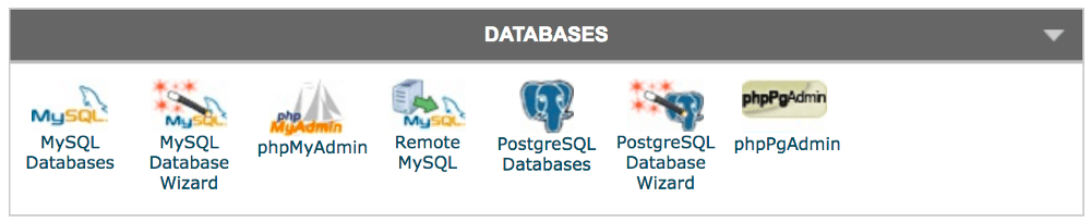
First, log into cPanel. From here, you should be able to find your list of MySQL databases under the Databases > MySQL Databases section:
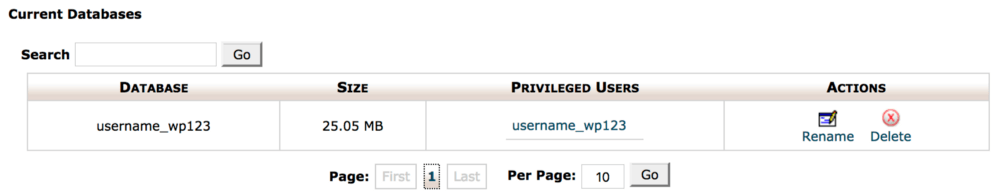
On this page, you should find a list of your existing databases. Some hosts name their databases differently, but typically include the prefix wp somewhere within the database name.
Identify your WordPress database, and copy and paste the name into a text file somewhere safe. Then, you can delete it by clicking the Delete button from the Actions column. This will completely wipe out your old WordPress database.
Step 2: Create a New Database
While you’ve just deleted the old database, it’s vital to set up a new one. Without a database, your WordPress website will not be able to load and you will not be able to access the dashboard to create any new content.
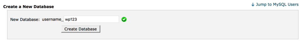
Once your old database is gone, it’s time to create a new one and set it up for WordPress. You should still be within the cPanel database page, so find the Create a New Database section. Here, you’ll complete the database name so it matches the old one:
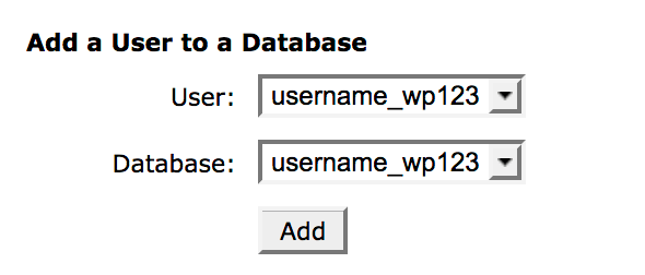
After clicking Create Database, the page should refresh and you’ll see the name pop up again under the Current Databases area. Next, find the Add a User to a Database section. You’ll need to add the old user with its permissions to the newly created database. Select the matching database and username in the drop-down menus and click Add User.
If you can’t find the old user, you may need to create it manually. This is easily possible under the Add a New User section. If possible, use the same username and password as the old database user. You can usually find these in your website’s wp-config.php file.
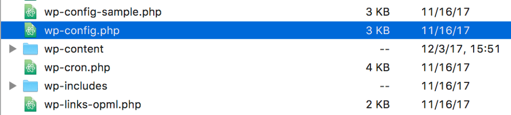
In your FTP program, navigate to your website’s public_html folder. From here you should see the WordPress root files. Right click on wp-config.php and choose View/Edit within your FTP program:
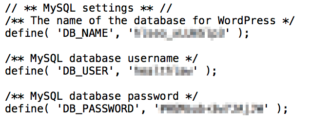
You don’t need to edit anything once you’re looking at the file. Instead, find the credentials for your old database user under MySQL Settings in the file.
Once you have these credentials, you can use them to recreate the correct user in MySQL. Don’t forget to follow the prior directions and add the user to the database once you’ve created it!
Step 3: Remove Unnecessary Files
With a clean database, you are now left with all the plugins, themes, and uploads you added to the old website. It’s important that you remove these, or you’ll have tons of unnecessary bloat on your new website. This isn’t preferable on a fresh site.
Now that your database is cleared up, you’ll want to turn your attention to your WordPress files. Most WordPress files remain the same between installations. What you’ll want to address are unique additions, such as plugins, themes, and media. These all exist within the wp-content folder.
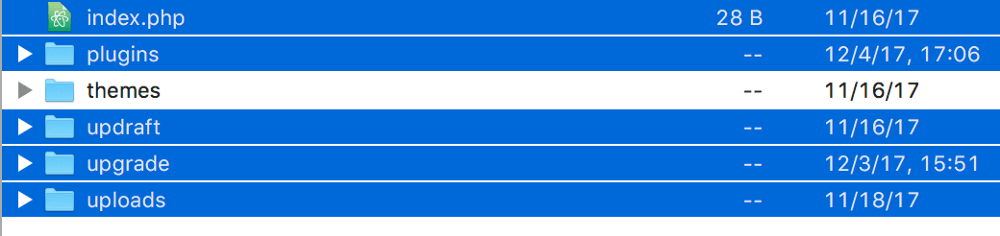
You can delete these via FTP. Log in using your favorite FTP application, and navigate to your WordPress’ root directory under public_html. Find the wp-content folder and navigate inside.
At this point you should see plugins, themes, and uploads folders. You may also see a few others. Select every folder except for themes and delete them all.
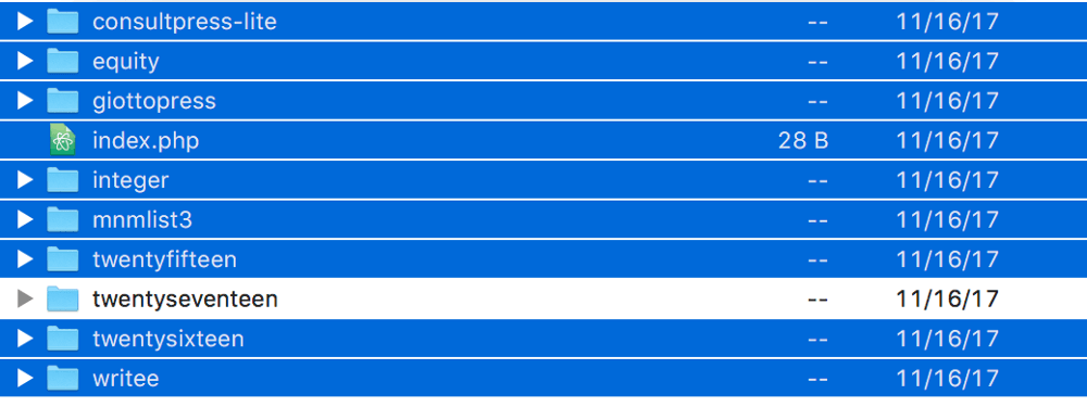
Next, navigate inside the themes folder. Choose the theme you’d like to keep, such as WordPress’ Twenty Seventeen. Select every theme folder except for your chosen theme, and remove them from the server.
At this point, you have now wiped out all unique elements related to your WordPress website. The database is completely empty, and all unique files have been removed. All that’s left is to reinstall WordPress from scratch!
Step 4: Run the WordPress Installation Script
At this point, everything in your WordPress site is sanitized and cleaned out. Unfortunately, if you leave it at this stage, you’ll not have a functional website — you need to rerun the WordPress installation script.
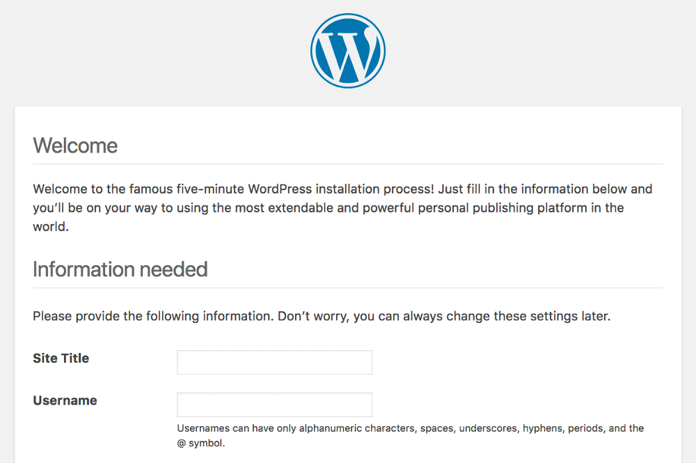
Finally, you’re ready to revert WordPress back to its default settings. You can load up the installation script by adding /wp-admin/install.php to the end of your domain name. You’ll need to pick out a few settings, such as language and your new login information:
Without this process, your database is completely blank. If you don’t run this script, WordPress will be unable to function. Once you’ve filled in the entire form, you can click Install WordPress. You’ll be greeted with a welcome message:
Simply click Log In and you’ll be on your way with a new WordPress website! This will regain your access to the site, and you’ll be working with a completely clean slate.
Conclusion
Resetting your WordPress website may not be the most thrilling task, but it is a good skill to have in your repertoire for fixing broken websites and cleaning up unnecessary files. Even if you use a plugin, it gives you the power to understand what is going on underneath the hood when resetting everything from scratch.
In this article, you learned how to do this manually in four steps:
Delete the WordPress database.
Create a new database.
Remove unnecessary files.
Run the WordPress installation script.
What questions do you have about resetting WordPress? Let us know in the comments section below!
This is a little article on how to start making pixel art, intended for those who are really starting out or never even opened a pixel art software. For now I’ll cover only the very basics, how to create a file, setup the canvas size, and work with a color limit.
This article was supported by Patreon! If you like what I’m doing here, please consider supporting me there 🙂
Before Starting
Before jumping into pixel art, remember: pixel art is just another art medium, like guache, oil painting, pencil, sculpture or its close cousin mosaic. To make good pixel art you need to be able to make good drawings. In general, this means studying anatomy, perspective, light and shadow, color theory and even art history, as these are all essential for making good pixel art.
Tools
You don’t need anything fancy to make good pixel art, and you can do fine even with just a good mouse and free software. My setup includes a small Wacom pen tablet, a good mouse, a good keyboard and my favorite software is Aseprite, but you should use whatever your’re most comfortable with.
Here’s a list of software commonly used for pixel art:
Aseprite: Great professional editor with many time-saving features (paid)
GraphicsGale: A classic, used in many games. It’s a little complex, but full of great features (free)
Photoshop: Powerful image editor not intended to make pixel art but you can set it up to use it (paid)
Aseprite
Aseprite is my favorite pixel art software right now. It’s incredibly powerful, packed with features and yet simple to use. I chose Aseprite as the software for this tutorial but I’m pretty sure you can adapt it to any other software you use with minimum changes. You can also get the free trial for Aseprite, but keep in mind it won’t save your files, which I guess it’s OK if you are just practicing.
Making a New File
Just click the “New File…” link in the home screen or go to File > New File so we can start drawing.
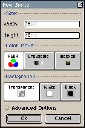
Let’s create a new file. 16 by 16 probably seems a little too small, but I think it’s a good starting point. Bigger resolutions can distract you from what you should focus now: understanding the interactions of pixels with their neighbors.
Aseprite ‘New Sprite’ dialog
You can leave the color mode in RGBA, that is the most simple and intuitive for now. Some pixel artists like to work with an indexed palette which allows some pretty cool color tricks, but comes with some drawbacks too.
Keep the background transparent or white, it won’t change much for now. Just make sure that Advanced Options is unchecked (but feel free to experiment with them later) and you are good to go!
Let’s Draw!
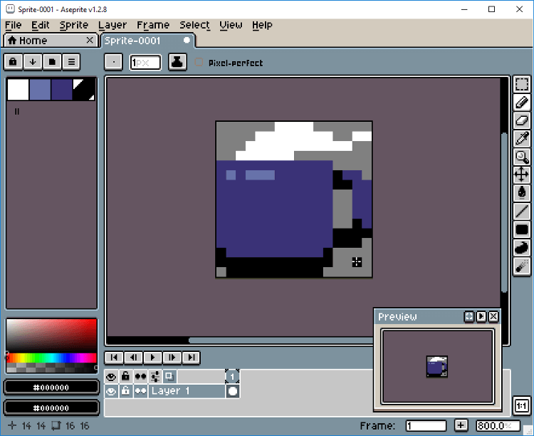
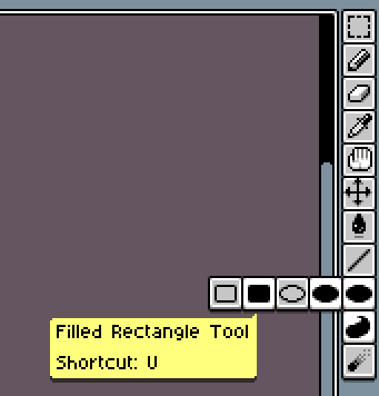
There are lots of toolbars and menus there, but don’t worry, we just need a few buttons for now. The main tool is the Pencil, that should always be kept with 1 pixel of width, and it will be how we place our pixels on the canvas. Just click the button, or press B, and click on the screen to place down a pixel of the selected color.
Aseprite workspace
On the left you can see your color palette, with some of the default colors. Let’s change those to another, simpler set. Click on the third icon on top of the color palette (Pressets) and choose ARQ4(a really good palette made by Endesga), that’s the one you will be using for your first sprite.
Now, only using the 4 colors on the top left, try drawing a mug.
Feel free to use mine as an inspiration, but also try making it unique. If you make a mistake, alt+click on an empty area or outside of your drawing and you will “pick” the transparent color and you can use it to erase pixels. Alternatively you can click on the Eraser or press E to select it.
You will probably notice that working in such a low resolution is very different from regular drawing. Everything needs to be calculated, and each pixel you place is a big choice you need to make. That’s the thing you will need to get used to.
You can also experiment with the other buttons in the toolbar. It’s worth noticing that some buttons will open more options when pressed. Just avoid the blur tool for now, as it adds more colors and we don’t want that yet.
Next, let’s make more sprites! Try drawing a skull, a sword and a human face. This time without my pixel art reference. If you feel that the sprites simply won’t fit in the canvas, that’s absolutely normal, try abstracting something to a single pixel and try again. It’s very hard to work with such a low resolution and it feels like a puzzle sometimes. Here’s another article I wrote about working with low resolutions for Kano: [link]
If you want, here’s my versions of those sprites, just please make sure to finish yours before looking at them [skull, sword and human face].
This is always a good exercise. If you want to keep practicing, try making even more drawings with those constrains.
Saving Your File
To save your file press Control+S (or go to File>Save As…), choose a file name and location and just hit save.
Don’t forget that in the trial version of Aseprite saving is disabled!
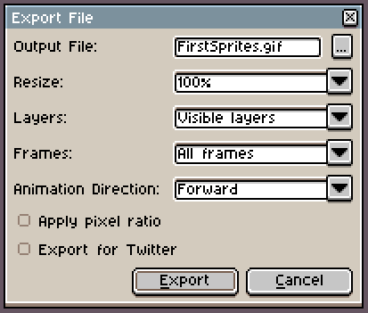
Aseprite Export File dialog
You will see that Aseprite can save in a variety of formats, but I always recommend keeping a .ase version of every file you make. Just like in Photoshop you would keep a .psd file. When exporting for web or games, you can use Control+Alt+Shif+S or File>Export.
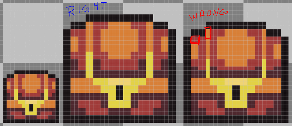
Why you should never resize a pixel art partially
Aseprite has this really good Resize feature in the export window. It only scales your sprite in round numbers, which is perfect. If you rescale your sprite 107%, for example, it will break pixels everywhere and it will be a mess, but if you scale it 200% each pixel will now be 2 pixels wide and tall, so it will look nice and sharp.
A Bigger Canvas
Now that you got the basics, like creating a new file, saving and drawing into the canvas, let’s try drawing on a slightly bigger canvas, 32 by 32 pixels. We’ll also use a bigger palette now, try the AAP-Micro12 (by AdigunPolack). This time we will draw a shovel.
Unlike the 16 by 16 sprite, we can actually fit some outlines here, so let’s start with that. Here’s my process breakdown:
Step 1: Lines
Step 1
This line style is what we call a pixel perfect line, it’s only 1 pixel wide and it connects diagonally with other pixels. When making lines like that we avoid unintentional edges, like here:
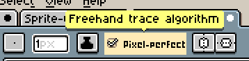
Aseprite also has a really good feature on the brush settings to do that almost automatically: with your brush tool selected, click the Pixel-perfect checkbox. Just don’t forget to toggle it off when not working with outlines because it will probably annoy you.
Aseprite Pixel perfect algorithm
Step 2: Base colors
Step 2
The good thing about having only so few colors to choose from is that you won’t be overwhelmed by too many options. That’s why it’s much harder to work with a lot of colors, if you have a color in your palette there’s no excuse not to use it at it’s best. Try to think of it as a puzzle, experiment a lot, even weird or unusual combinations until you find what you believe is the “best match” for each area.
Step 3: Shading
Step 3
Use your palette to make light and shadow in creative ways. Since you are working with a very restricted palette, you won’t have every hue with different brightness, so you will have to improvise.
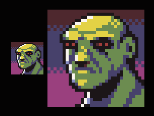
Improvising shade tones with different hues
In the example on the left I’m using the same palette you are, the AAP-Mini12. When I drew this green dude I didn’t have any light green color, so I went with the nearest hue I had available, which was yellow. The same thing happened with the shadow, I chose blue because it was the closest dark one. But what if I went the other way? I could get a brighter blue and darker red, right? Well, not really:
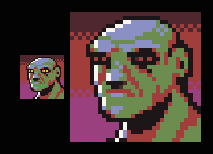
Shade tones using inverted hue
It’s a cool effect, but clearly there’s something wrong. Usually you will want the cold hues to be your shadows and warm hues to be your key light, or they might look weird. This is not a stone-written-rule or anything, there are many exceptions, but when not sure, just go with it.
Step 4: Anti-alias and polish
Step 4
This is the part of the drawing where you try to make the pixels a little less “pointy”. Manual anti alias is a complex subject, and we probably will need a whole article to discuss just that, but the theory is, you will use mid tones to simulate “half pixels” and soften the edges. But don’t worry too much about this yet, for now focus on making your sprite as readable as possible.
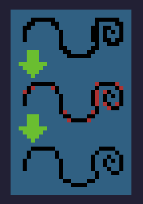
Another good idea in this step is to hunt down some orphan pixels to reduce noise. Orphan pixels are pixels that are not part of a bigger group of pixels of the same color and are not part of the anti-alias, like this:
Removing orphan pixels
You see the little 1-pixel-islands on the left? Those are orphan pixels, as you can see the planet looks much better after we merge those pixels with some other nearby pixels of the same color.
And what about the stars in that example? Well, they are there to prove that orphan pixels are not always bad, those stars work exactly as intended, creating a noise texture and bringing up the contrast in the background.
The idea is not to mindlessly remove orphan pixels, but to through them and ask yourself: does this pixel really need to be alone?
Now What?
Now it’s time for you to experiment with more colors and bigger resolutions! But go slowly, maybe 48 by 48 and 16 colors and so on. If you are really starting out I would avoid animation for now and focus on getting comfortable with static images first.
I selected some other pixel art guides that I really like if you want to do some research:
I also plan to make more articles like this and keep writing about the individual steps on how I like to make pixel art. So keep an eye on my Patreon to get the next articles.
The 5 Computer Vision Techniques That Will Change How You See The World
Computer Vision is one of the hottest research fields within Deep Learning at the moment. It sits at the intersection of many academic subjects, such as Computer Science (Graphics, Algorithms, Theory, Systems, Architecture), Mathematics (Information Retrieval, Machine Learning), Engineering (Robotics, Speech, NLP, Image Processing), Physics (Optics), Biology (Neuroscience), and Psychology (Cognitive Science). As Computer Vision represents a relative understanding of visual environments and their contexts, many scientists believe the field paves the way towards Artificial General Intelligence due to its cross-domain mastery.
So what is Computer Vision? Here are a couple of formal textbook definitions:
“the construction of explicit, meaningful descriptions of physical objects from images” (Ballard & Brown, 1982)
“computing properties of the 3D world from one or more digital images” (Trucco & Verri, 1998)
“to make useful decisions about real physical objects and scenes based on sensed images” (Sockman & Shapiro, 2001)
Why study Computer Vision? The most obvious answer is that there’s a fast-growing collection of useful applications derived from this field of study. Here are just a handful of them:
Face recognition: Snapchat and Facebook use face-detection algorithms to apply filters and recognize you in pictures.
Image retrieval: Google Images uses content-based queries to search relevant images. The algorithms analyze the content in the query image and return results based on best-matched content.
Gaming and controls: A great commercial product in gaming that uses stereo vision is Microsoft Kinect.
Surveillance: Surveillance cameras are ubiquitous at public locations and are used to detect suspicious behaviors.
Biometrics: Fingerprint, iris and face matching remains some common methods in biometric identification.
Smart cars: Vision remains the main source of information to detect traffic signs and lights and other visual features.
I recently finished Stanford’s wonderful CS231n course on using Convolutional Neural Networks for visual recognition. Visual recognition tasks such as image classification, localization, and detection are key components of Computer vision. Recent developments in neural networks and deep learning approaches have greatly advanced the performance of these state-of-the-art visual recognition systems. The course is a phenomenal resource that taught me the details of deep learning architectures being used in cutting-edge computer vision research. In this article, I want to share the 5 major computer vision techniques I’ve learned as well as major deep learning models and applications using each of them.
1 — Image Classification
The problem of Image Classification goes like this: Given a set of images that are all labeled with a single category, we’re asked to predict these categories for a novel set of test images and measure the accuracy of the predictions. There are a variety of challenges associated with this task, including viewpoint variation, scale variation, intra-class variation, image deformation, image occlusion, illumination conditions, and background clutter.
How might we go about writing an algorithm that can classify images into distinct categories? Computer Vision researchers have come up with a data-driven approach to solve this. Instead of trying to specify what every one of the image categories of interest look like directly in code, they provide the computer with many examples of each image class and then develop learning algorithms that look at these examples and learn about the visual appearance of each class. In other words, they first accumulate a training dataset of labeled images, then feed it to the computer to process the data.
Given that fact, the complete image classification pipeline can be formalized as follows:
Our input is a training dataset that consists of N images, each labeled with one of K different classes.
Then, we use this training set to train a classifier to learn what every one of the classes looks like.
In the end, we evaluate the quality of the classifier by asking it to predict labels for a new set of images that it’s never seen before. We’ll then compare the true labels of these images to the ones predicted by the classifier.
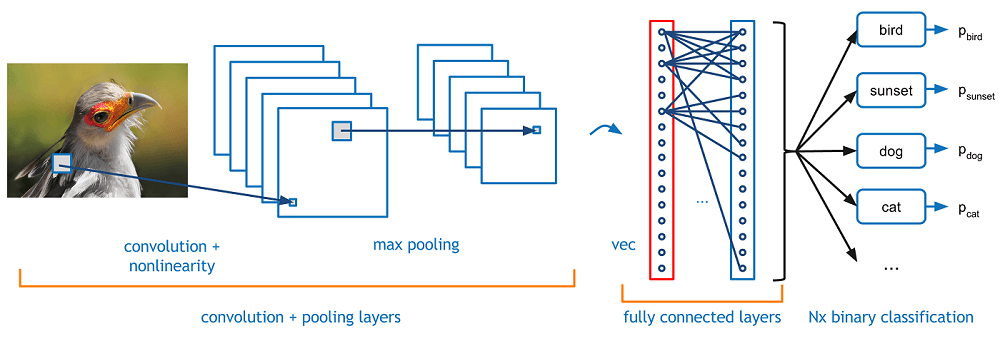
The most popular architecture used for image classification is Convolutional Neural Networks (CNNs). A typical use case for CNNs is where you feed the network images and the network classifies the data. CNNs tend to start with an input “scanner” which isn’t intended to parse all the training data at once. For example, to input an image of 100 x 100 pixels, you wouldn’t want a layer with 10,000 nodes. Rather, you create a scanning input layer of say 10 x 10 which you feed the first 10 x 10 pixels of the image. Once you passed that input, you feed it the next 10 x 10 pixels by moving the scanner one pixel to the right. This technique is known as sliding windows.
This input data is then fed through convolutional layers instead of normal layers. Each node only concerns itself with close neighboring cells. These convolutional layers also tend to shrink as they become deeper, mostly by easily divisible factors of the input. Besides these convolutional layers, they also often feature pooling layers. Pooling is a way to filter out details: a commonly found pooling technique is max pooling, where we take, say, 2 x 2 pixels and pass on the pixel with the most amount of a certain attribute.
Most image classification techniques nowadays are trained on ImageNet, a dataset with approximately 1.2 million high-resolution training images. Test images will be presented with no initial annotation (no segmentation or labels), and algorithms will have to produce labelings specifying what objects are present in the images. Some of the best existing computer vision methods were tried on this dataset by leading computer vision groups from Oxford, INRIA, and XRCE.Typically, computer vision systems use complicated multi-stage pipelines, and the early stages are typically hand-tuned by optimizing a few parameters.
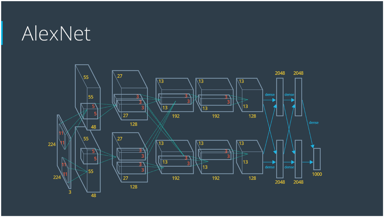
The winner of the 1st ImageNet competition, Alex Krizhevsky (NIPS 2012), developed a very deep convolutional neural net of the type pioneered by Yann LeCun. Its architecture includes 7 hidden layers, not counting some max pooling layers. The early layers were convolutional, while the last 2 layers were globally connected. The activation functions were rectified linear units in every hidden layer. These train much faster and are more expressive than logistic units. In addition to that, it also uses competitive normalization to suppress hidden activities when nearby units have stronger activities. This helps with variations in intensity.
In terms of hardware requirements, Alex uses a very efficient implementation of convolutional nets on 2 Nvidia GTX 580 GPUs (over 1000 fast little cores). The GPUs are very good for matrix-matrix multiplies and also have very high bandwidth to memory. This allows him to train the network in a week and makes it quick to combine results from 10 patches at test time. We can spread a network over many cores if we can communicate the states fast enough. As cores get cheaper and datasets get bigger, big neural nets will improve faster than old-fashioned computer vision systems. Since AlexNet, there have been multiple new models using CNN as their backbone architecture and achieving excellent results in ImageNet: ZFNet (2013), GoogLeNet (2014), VGGNet (2014), ResNet (2015), DenseNet (2016) etc.
2 — Object Detection
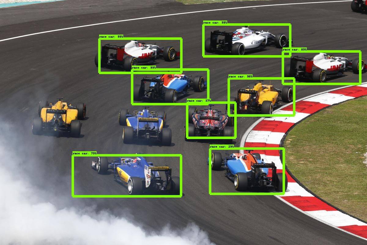
The task to define objects within images usually involves outputting bounding boxes and labels for individual objects. This differs from the classification / localization task by applying classification and localization to many objects instead of just a single dominant object. You only have 2 classes of object classification, which means object bounding boxes and non-object bounding boxes. For example, in car detection, you have to detect all cars in a given image with their bounding boxes.
If we use the Sliding Window technique like the way we classify and localize images, we need to apply a CNN to many different crops of the image. Because CNN classifies each crop as object or background, we need to apply CNN to huge numbers of locations and scales, which is very computationally expensive!
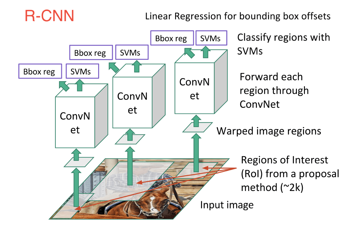
In order to cope with this, neural network researchers have proposed to use regions instead, where we find “blobby” image regions that are likely to contain objects. This is relatively fast to run. The first model that kicked things off was R-CNN(Region-based Convolutional Neural Network). In a R-CNN, we first scan the input image for possible objects using an algorithm called Selective Search, generating ~2,000 region proposals. Then we run a CNN on top of each of these region proposals. Finally, we take the output of each CNN and feed it into an SVM to classify the region and a linear regression to tighten the bounding box of the object.
Essentially, we turned object detection into an image classification problem. However, there are some problems — the training is slow, a lot of disk space is required, and inference is also slow.
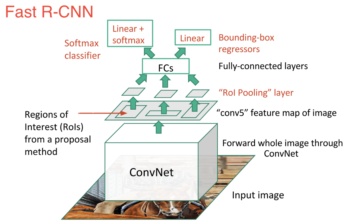
An immediate descendant to R-CNN is Fast R-CNN, which improves the detection speed through 2 augmentations: 1) Performing feature extraction before proposing regions, thus only running one CNN over the entire image, and 2) Replacing SVM with a softmax layer, thus extending the neural network for predictions instead of creating a new model.
Fast R-CNN performed much better in terms of speed, because it trains just one CNN for the entire image. However, the selective search algorithm is still taking a lot of time to generate region proposals.
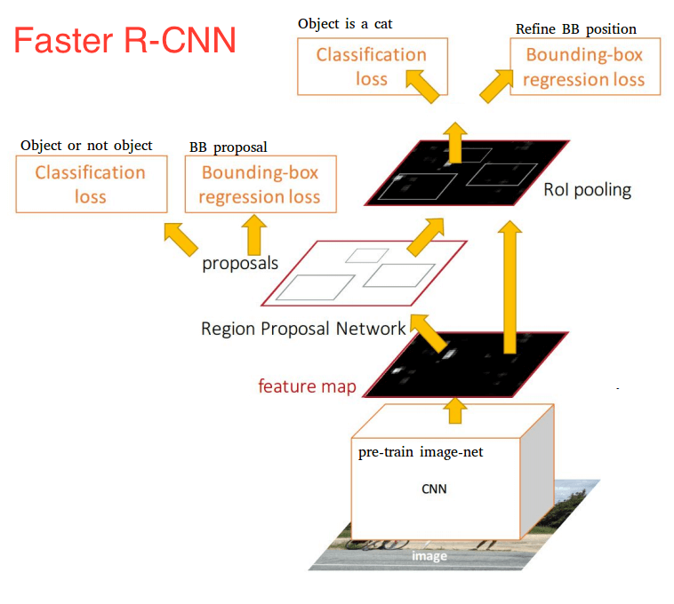
Thus comes the invention of Faster R-CNN, which now is a canonical model for deep learning-based object detection. It replaces the slow selective search algorithm with a fast neural network by inserting a Region Proposal Network (RPN) to predict proposals from features. The RPN is used to decide “where” to look in order to reduce the computational requirements of the overall inference process. The RPN quickly and efficiently scans every location in order to assess whether further processing needs to be carried out in a given region. It does that by outputting k bounding box proposals each with 2 scores representing the probability of object or not at each location.
Once we have our region proposals, we feed them straight into what is essentially a Fast R-CNN. We add a pooling layer, some fully-connected layers, and finally a softmax classification layer and bounding box regressor.
Altogether, Faster R-CNN achieved much better speeds and higher accuracy. It’s worth noting that although future models did a lot to increase detection speeds, few models managed to outperform Faster R-CNN by a significant margin. In other words, Faster R-CNN may not be the simplest or fastest method for object detection, but it’s still one of the best performing.
Major Object Detection trends in recent years have shifted towards quicker, more efficient detection systems. This was visible in approaches like You Only Look Once (YOLO), Single Shot MultiBox Detector (SSD), and Region-Based Fully Convolutional Networks (R-FCN) as a move towards sharing computation on a whole image. Hence, these approaches differentiate themselves from the costly subnetworks associated with the 3 R-CNN techniques. The main rationale behind these trends is to avoid having separate algorithms focus on their respective subproblems in isolation, as this typically increases training time and can lower network accuracy.
3 — Object Tracking
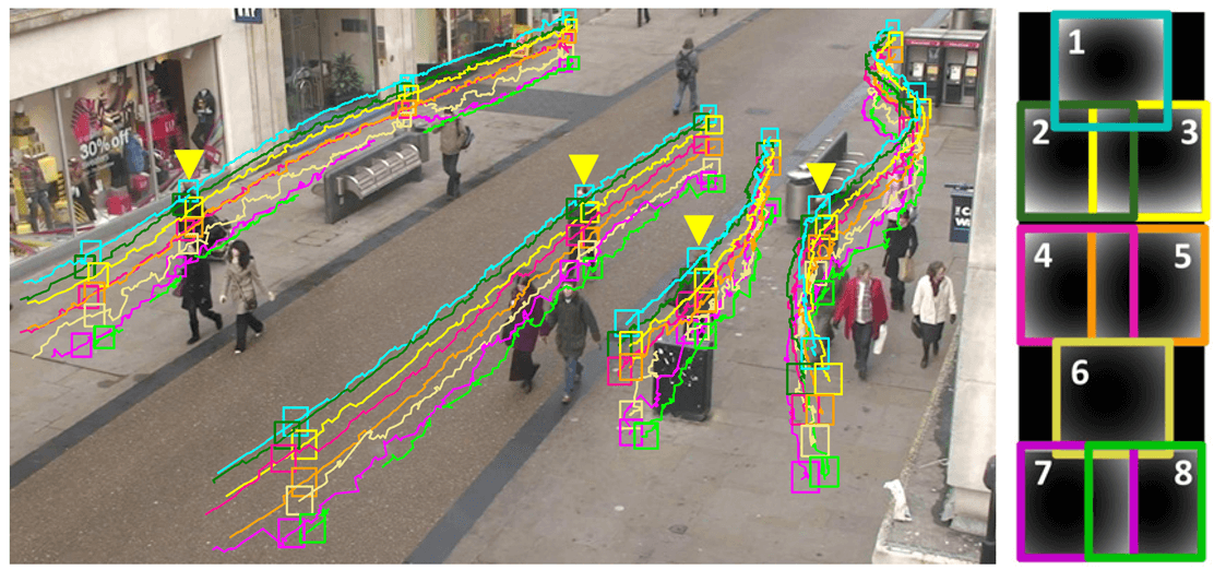
Object Tracking refers to the process of following a specific object of interest, or multiple objects, in a given scene. It traditionally has applications in video and real-world interactions where observations are made following an initial object detection. Now, it’s crucial to autonomous driving systems such as self-driving vehicles from companies like Uber and Tesla.
Object Tracking methods can be divided into 2 categories according to the observation model: generative method and discriminative method. The generative method uses the generative model to describe the apparent characteristics and minimizes the reconstruction error to search the object, such as PCA. The discriminative method can be used to distinguish between the object and the background, its performance is more robust, and it gradually becomes the main method in tracking. Discriminative method is also referred to as Tracking-by-Detection, and deep learning belongs to this category. To achieve the tracking by detection, we detect candidate objects for all frames and use deep learning to recognize the wanted object from the candidates. There are 2 kinds of basic network models that can be used: stacked auto encoders (SAE) and convolutional neural network (CNN).
The most popular deep network for tracking tasks using SAE is Deep Learning Tracker, which proposes offline pre-training and online fine-tuning the net. The process works like this:
Off-line unsupervised pre-train the stacked denoising auto-encoder using large-scale natural image datasets to obtain the general object representation. Stacked denoising auto-encoder can obtain more robust feature expression ability by adding noise in input images and reconstructing the original images.
Combine the coding part of the pre-trained network with a classifier to get the classification network, then use the positive and negative samples obtained from the initial frame to fine-tune the network, which can discriminate the current object and background. DLT uses particle filter as the motion model to produce candidate patches of the current frame. The classification network outputs the probability scores for these patches, meaning the confidence of their classifications, then chooses the highest of these patches as the object.
In the model updating, DLT uses the way of limited threshold.
Because of its superiority in image classification and object detection, CNN has become the mainstream deep model in computer vision and in visual tracking. Generally speaking, a large-scale CNN can be trained both as a classifier and as a tracker. 2 representative CNN-based tracking algorithms are fully-convolutional network tracker(FCNT) and multi-domain CNN(MD Net).
FCNT analyzes and takes advantage of the feature maps of the VGG model successfully, which is a pre-trained ImageNet, and results in the following observations:
CNN feature maps can be used for localization and tracking.
Many CNN feature maps are noisy or un-related for the task of discriminating a particular object from its background.
Higher layers capture semantic concepts on object categories, whereas lower layers encode more discriminative features to capture intra-class variation.
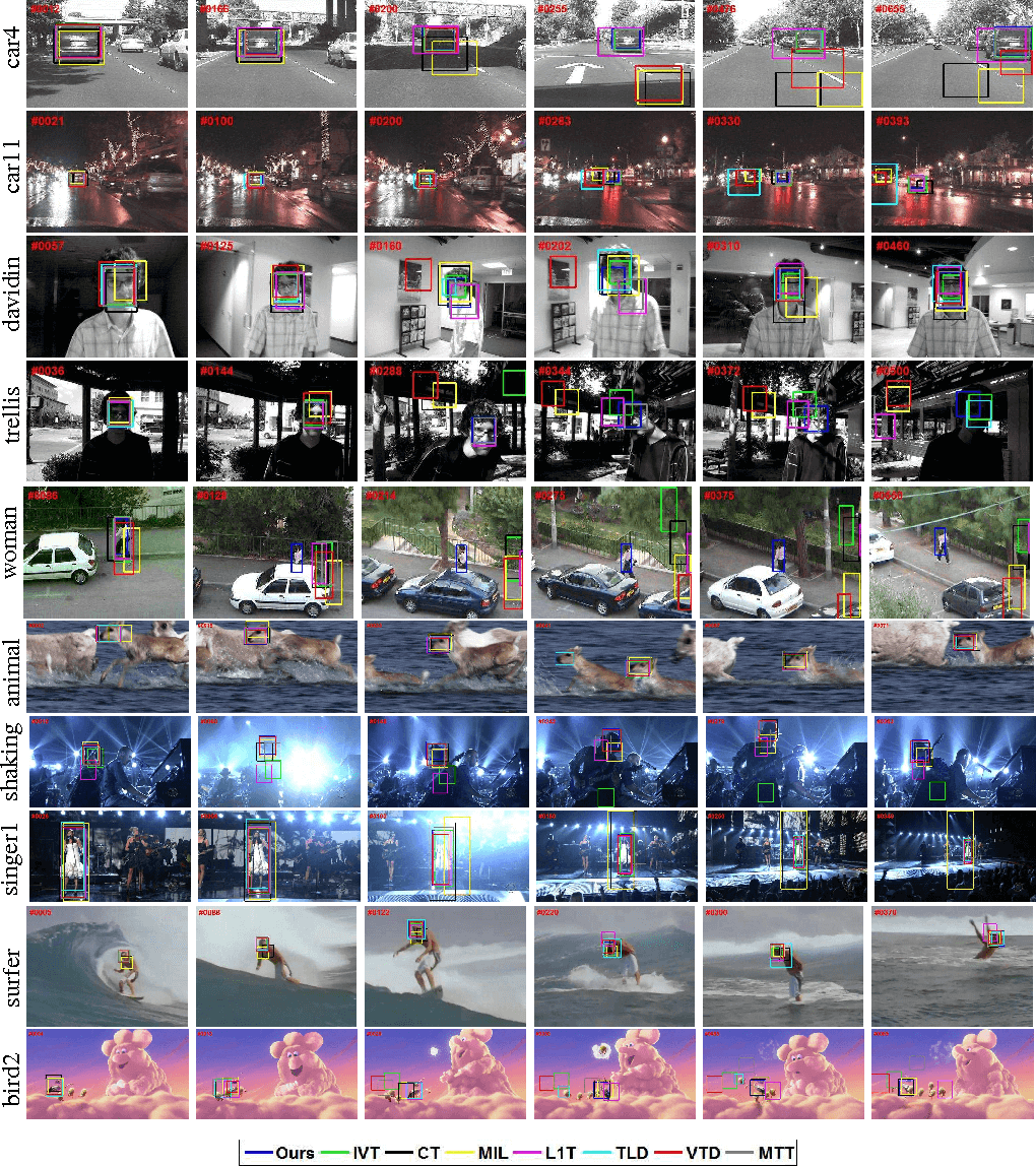
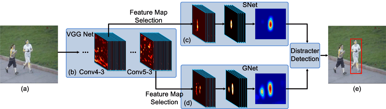
Because of these observations, FCNT designs the feature selection network to select the most relevant feature maps on the conv4–3 and conv5–3 layers of the VGG network. Then in order to avoid overfitting on noisy ones, it also designs extra two channels (called SNet and GNet) for the selected feature maps from two layers’ separately. The GNet captures the category information of the object, while the SNet discriminates the object from a background with a similar appearance. Both of the networks are initialized with the given bounding-box in the first frame to get heat maps of the object, and for new frames, a region of interest (ROI) centered at the object location in the last frame is cropped and propagated. At last, through SNet and GNet, the classifier gets two heat maps for prediction, and the tracker decides which heat map will be used to generate the final tracking result according to whether there are distractors. The pipeline of FCNT is shown below.
Different from the idea of FCNT, MD Net uses all the sequences of a video to to track movements in them. The networks mentioned above use irrelevant image data to reduce the training demand of tracking data, and this idea has some deviation from tracking. The object of one class in this video can be the background in another video, so MD Net proposes the idea of multi-domain to distinguish the object and background in every domain independently. And a domain indicates a set of videos that contain the same kind of object.
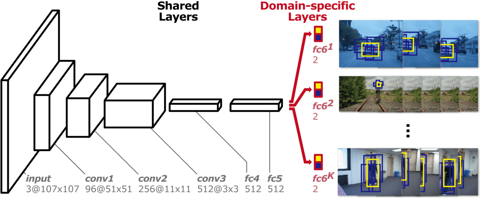
As shown below, MD Net is divided into 2 parts: the shared layers and the K branches of domain-specific layers. Each branch contains a binary classification layer with softmax loss, which is used to distinguish the object and background in each domain, and the shared layers sharing with all domains to ensure the general representation.
In recent years, deep learning researchers have tried different ways to adapt to features of the visual tracking task. There are many directions that have been explored: applying other network models such as Recurrent Neural Net and Deep Belief Net, designing the network structure to adapt to video processing and end-to-end learning, optimizing the process, structure, and parameters, or even combining deep learning with traditional methods of computer vision or approaches in other fields such as Language Processing and Speech Recognition.
4 — Semantic Segmentation
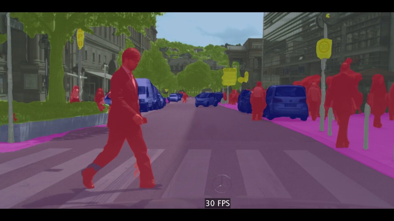
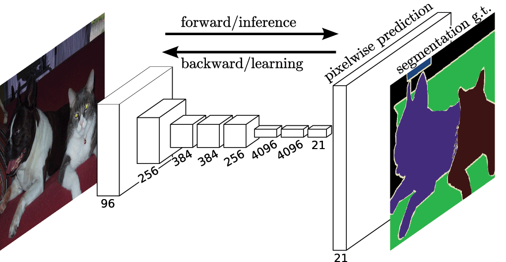
Central to Computer Vision is the process of Segmentation, which divides whole images into pixel groupings which can then be labelled and classified. Particularly, Semantic Segmentation tries to semantically understand the role of each pixel in the image (e.g. is it a car, a motorbike, or some other type of class?). For example, in the picture above, apart from recognizing the person, the road, the cars, the trees, etc., we also have to delineate the boundaries of each object. Therefore, unlike classification, we need dense pixel-wise predictions from our models.
As with other computer vision tasks, CNNs have had enormous success on segmentation problems. One of the popular initial approaches was patch classification through sliding window, where each pixel was separately classified into classes using a patch of images around it. This, however, is very inefficient computationally because we don’t reuse the shared features between overlapping patches.
The solution, instead, is UC Berkeley’s Fully Convolutional Networks(FCN), which popularized end-to-end CNN architectures for dense predictions without any fully connected layers. This allowed segmentation maps to be generated for images of any size and was also much faster compared to the patch classification approach. Almost all subsequent t approaches on semantic segmentation adopted this paradigm.
However, one problem remains: convolutions at original image resolution will be very expensive. To deal with this, FCN uses downsampling and upsampling inside the network. The downsampling layer is known as striped convolution, while the upsampling layer is known as transposed convolution.
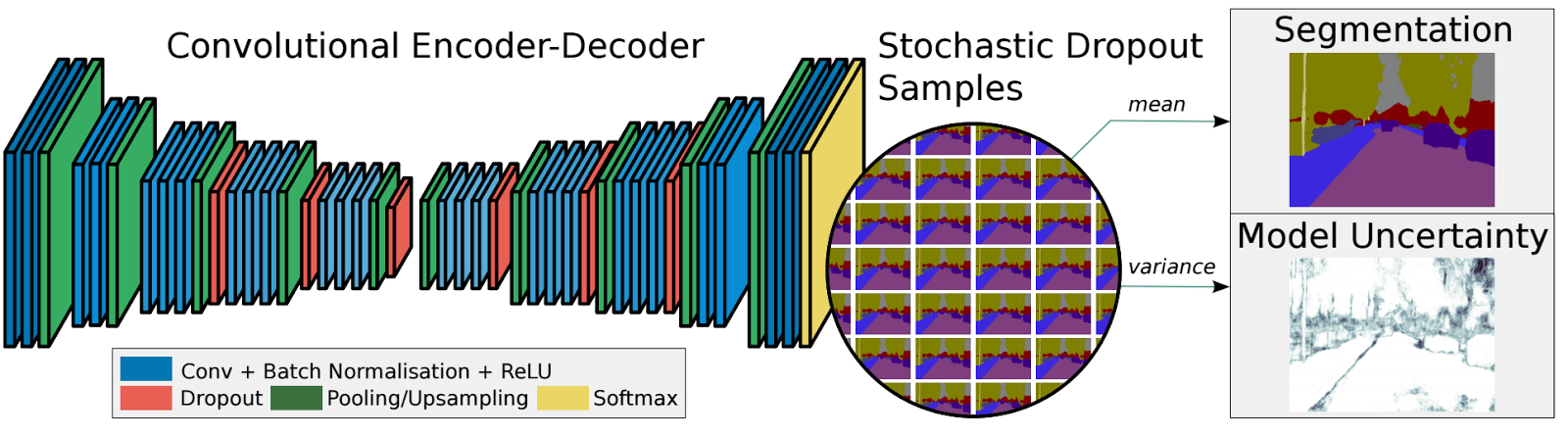
Despite the upsampling/downsampling layers, FCN produces coarse segmentation maps because of information loss during pooling. SegNet is a more memory efficient architecture than FCN that uses-max pooling and an encoder-decoder framework. In SegNet, shortcut/skip connections are introduced from higher resolution feature maps to improve the coarseness of upsampling/downsampling.
Recent research in Semantic Segmentation all relies heavily on fully convolutional networks, such as Dilated Convolutions, DeepLab, and RefineNet.
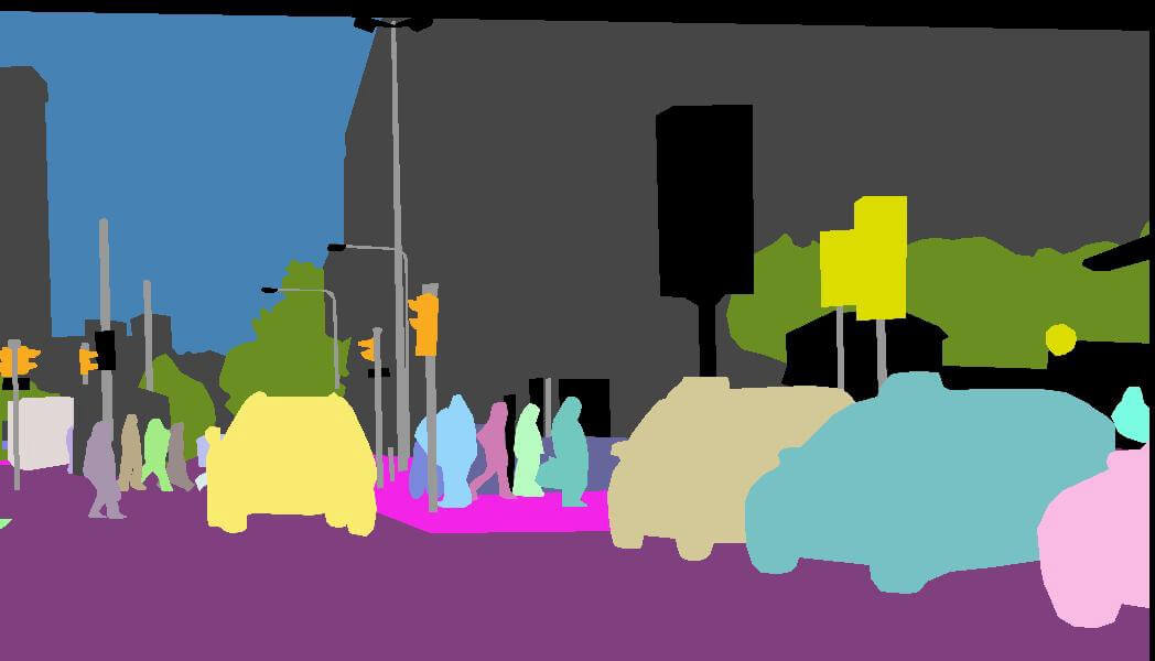
5 — Instance Segmentation
Beyond Semantic Segmentation, Instance Segmentation segments different instances of classes, such as labelling 5 cars with 5 different colors. In classification, there’s generally an image with a single object as the focus and the task is to say what that image is. But in order to segment instances, we need to carry out far more complex tasks. We see complicated sights with multiple overlapping objects and different backgrounds, and we not only classify these different objects but also identify their boundaries, differences, and relations to one another!
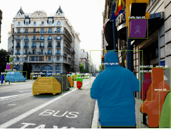
So far, we’ve seen how to use CNN features in many interesting ways to effectively locate different objects in an image with bounding boxes. Can we extend such techniques to locate exact pixels of each object instead of just bounding boxes? This instance segmentation problem is explored at Facebook AI using an architecture known as Mask R-CNN.
Much like Fast R-CNN, and Faster R-CNN, Mask R-CNN’s underlying intuition is straightforward Given that Faster R-CNN works so well for object detection, could we extend it to also carry out pixel-level segmentation?
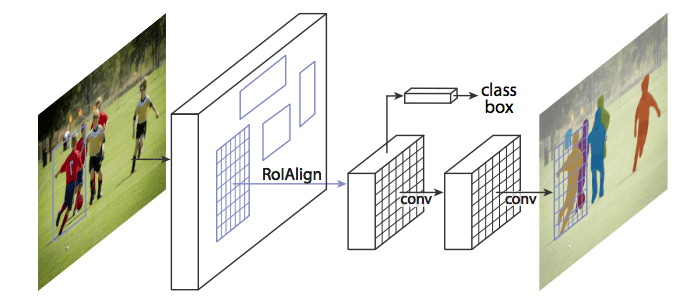
Mask R-CNN does this by adding a branch to Faster R-CNN that outputs a binary mask that says whether or not a given pixel is part of an object. The branch is a Fully Convolutional Network on top of a CNN-based feature map. Given the CNN Feature Map as the input, the network outputs a matrix with 1s on all locations where the pixel belongs to the object and 0s elsewhere (this is known as a binary mask).
Additionally, when run without modifications on the original Faster R-CNN architecture, the regions of the feature map selected by RoIPool (Region of Interests Pool) were slightly misaligned from the regions of the original image. Since image segmentation requires pixel-level specificity, unlike bounding boxes, this naturally led to inaccuracies. Mask R-CNN solves this problem by adjusting RoIPool to be more precisely aligned using a method known as RoIAlign (Region of Interests Align). Essentially, RoIAlign uses bilinear interpolation to avoid error in rounding, which causes inaccuracies in detection and segmentation.
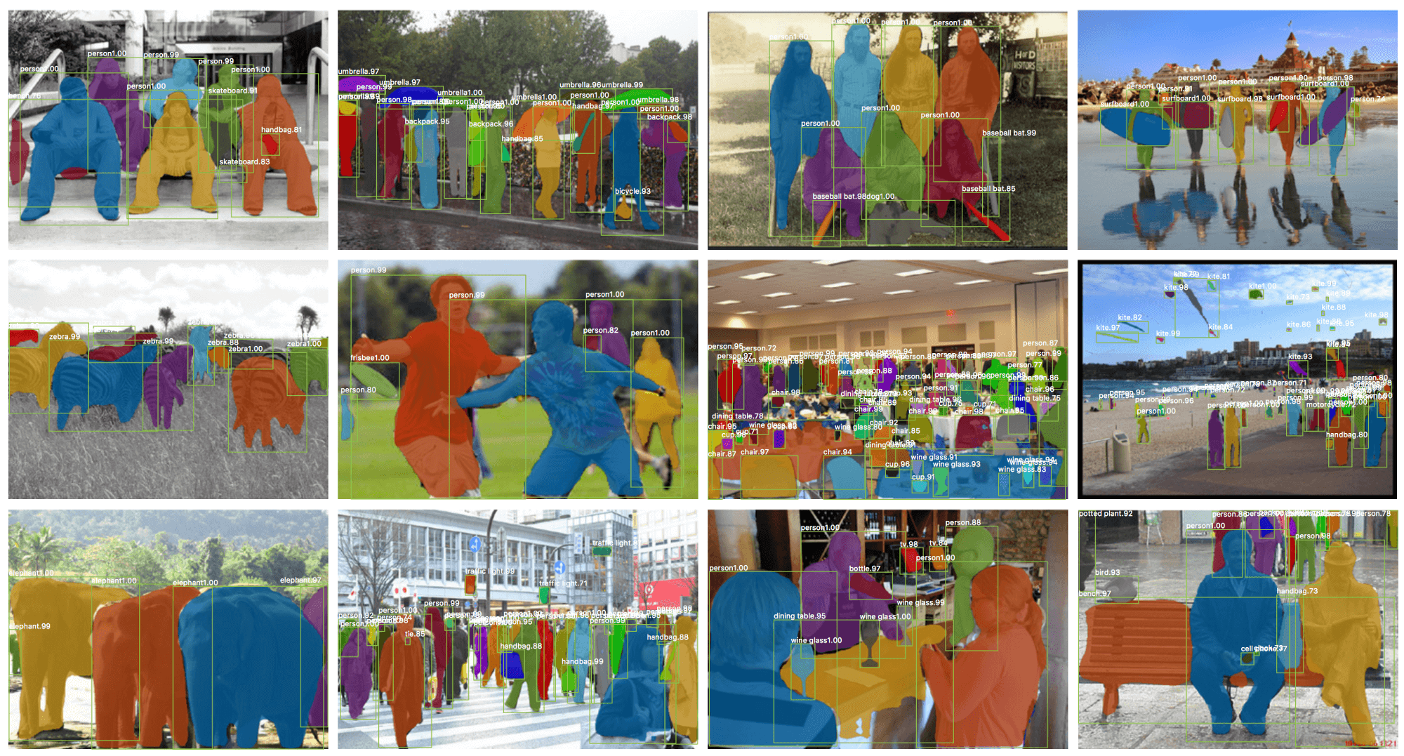
Once these masks are generated, Mask R-CNN combines them with the classifications and bounding boxes from Faster R-CNN to generate such wonderfully precise segmentations:
Conclusion
These 5 major computer vision techniques can help a computer extract, analyze, and understand useful information from a single or a sequence of images. There are many other advanced techniques that I haven’t touched, including style transfer, colorization, action recognition, 3D objects, human pose estimation, and more. Indeed, the field of Computer Vision is too expensive to cover in depth, and I would encourage you to explore it further, whether through online courses, blog tutorials, or formal documents. I’d highly recommend CS231n for starters, as you’ll learn to implement, train, and debug your own neural networks. As a bonus, you can get all the lecture slides and assignment guidelines from my GitHub repository. I hope it’ll guide you in the quest of changing how to see the world!
Computers are great at working with structured data like spreadsheets and database tables. But us humans usually communicate in words, not in tables. That’s unfortunate for computers.
Unfortunately we don’t live in this alternate version of history where all data is structured.
A lot of information in the world is unstructured — raw text in English or another human language. How can we get a computer to understand unstructured text and extract data from it?
Natural Language Processing, or NLP, is the sub-field of AI that is focused on enabling computers to understand and process human languages. Let’s check out how NLP works and learn how to write programs that can extract information out of raw text using Python!
Note: If you don’t care how NLP works and just want to cut and paste some code, skip way down to the section called “Coding the NLP Pipeline in Python”.
Can Computers Understand Language?
As long as computers have been around, programmers have been trying to write programs that understand languages like English. The reason is pretty obvious — humans have been writing things down for thousands of years and it would be really helpful if a computer could read and understand all that data.
Computers can’t yet truly understand English in the way that humans do — but they can already do a lot! In certain limited areas, what you can do with NLP already seems like magic. You might be able to save a lot of time by applying NLP techniques to your own projects.
And even better, the latest advances in NLP are easily accessible through open source Python libraries like spaCy, textacy, and neuralcoref. What you can do with just a few lines of python is amazing.
Extracting Meaning from Text is Hard
The process of reading and understanding English is very complex — and that’s not even considering that English doesn’t follow logical and consistent rules. For example, what does this news headline mean?
“Environmental regulators grill business owner over illegal coal fires.”
Are the regulators questioning a business owner about burning coal illegally? Or are the regulators literally cooking the business owner? As you can see, parsing English with a computer is going to be complicated.
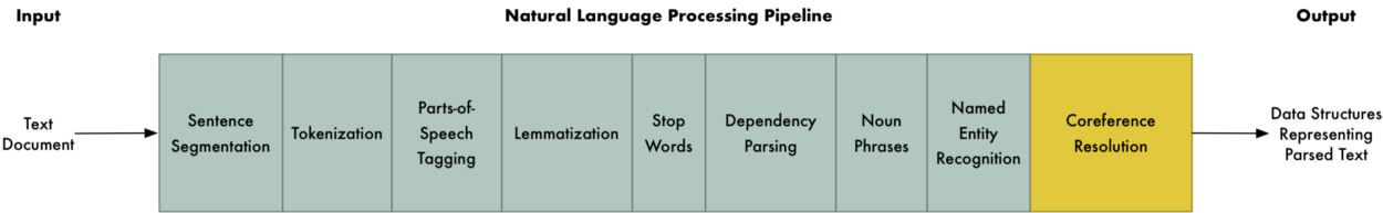
Doing anything complicated in machine learning usually means building a pipeline. The idea is to break up your problem into very small pieces and then use machine learning to solve each smaller piece separately. Then by chaining together several machine learning models that feed into each other, you can do very complicated things.
And that’s exactly the strategy we are going to use for NLP. We’ll break down the process of understanding English into small chunks and see how each one works.
Building an NLP Pipeline, Step-by-Step
Let’s look at a piece of text from Wikipedia:
London is the capital and most populous city of England and the United Kingdom. Standing on the River Thames in the south east of the island of Great Britain, London has been a major settlement for two millennia. It was founded by the Romans, who named it Londinium.
This paragraph contains several useful facts. It would be great if a computer could read this text and understand that London is a city, London is located in England, London was settled by Romans and so on. But to get there, we have to first teach our computer the most basic concepts of written language and then move up from there.
Step 1: Sentence Segmentation
The first step in the pipeline is to break the text apart into separate sentences. That gives us this:
“London is the capital and most populous city of England and the United Kingdom.”
“Standing on the River Thames in the south east of the island of Great Britain, London has been a major settlement for two millennia.”
“It was founded by the Romans, who named it Londinium.”
We can assume that each sentence in English is a separate thought or idea. It will be a lot easier to write a program to understand a single sentence than to understand a whole paragraph.
Coding a Sentence Segmentation model can be as simple as splitting apart sentences whenever you see a punctuation mark. But modern NLP pipelines often use more complex techniques that work even when a document isn’t formatted cleanly.
Step 2: Word Tokenization
Now that we’ve split our document into sentences, we can process them one at a time. Let’s start with the first sentence from our document:
“London is the capital and most populous city of England and the United Kingdom.”
The next step in our pipeline is to break this sentence into separate words or tokens. This is called tokenization. This is the result:
Tokenization is easy to do in English. We’ll just split apart words whenever there’s a space between them. And we’ll also treat punctuation marks as separate tokens since punctuation also has meaning.
Step 3: Predicting Parts of Speech for Each Token
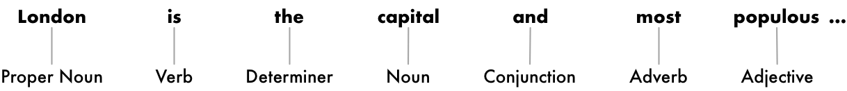
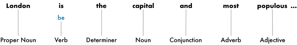
Next, we’ll look at each token and try to guess its part of speech — whether it is a noun, a verb, an adjective and so on. Knowing the role of each word in the sentence will help us start to figure out what the sentence is talking about.
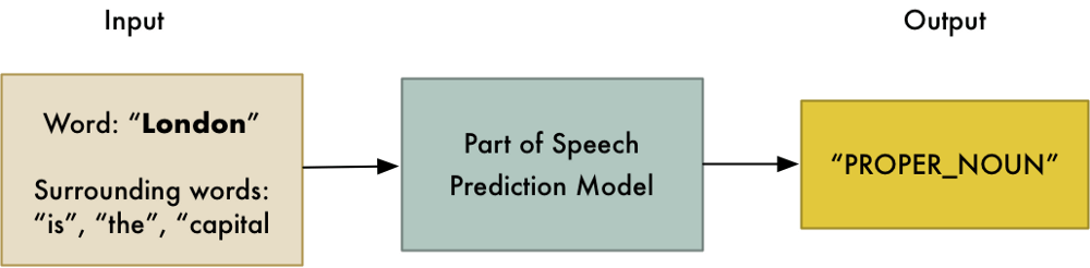
We can do this by feeding each word (and some extra words around it for context) into a pre-trained part-of-speech classification model:
The part-of-speech model was originally trained by feeding it millions of English sentences with each word’s part of speech already tagged and having it learn to replicate that behavior.
Keep in mind that the model is completely based on statistics — it doesn’t actually understand what the words mean in the same way that humans do. It just knows how to guess a part of speech based on similar sentences and words it has seen before.
After processing the whole sentence, we’ll have a result like this:
With this information, we can already start to glean some very basic meaning. For example, we can see that the nouns in the sentence include “London” and “capital”, so the sentence is probably talking about London.
Step 4: Text Lemmatization
In English (and most languages), words appear in different forms. Look at these two sentences:
I had a pony.
I had two ponies.
Both sentences talk about the noun pony, but they are using different inflections. When working with text in a computer, it is helpful to know the base form of each word so that you know that both sentences are talking about the same concept. Otherwise the strings “pony” and “ponies” look like two totally different words to a computer.
In NLP, we call finding this process lemmatization — figuring out the most basic form or lemma of each word in the sentence.
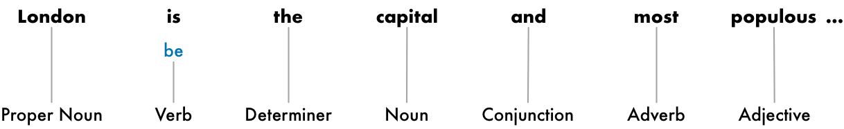
The same thing applies to verbs. We can also lemmatize verbs by finding their root, unconjugated form. So “I had two ponies” becomes “I [have] two [pony].”
Lemmatization is typically done by having a look-up table of the lemma forms of words based on their part of speech and possibly having some custom rules to handle words that you’ve never seen before.
Here’s what our sentence looks like after lemmatization adds in the root form of our verb:
The only change we made was turning “is” into “be”.
Step 5: Identifying Stop Words
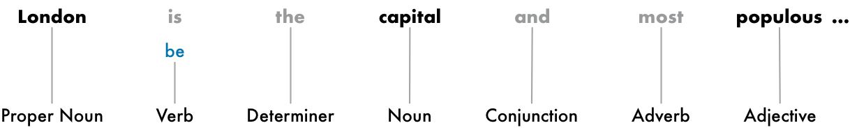
Next, we want to consider the importance of a each word in the sentence. English has a lot of filler words that appear very frequently like “and”, “the”, and “a”. When doing statistics on text, these words introduce a lot of noise since they appear way more frequently than other words. Some NLP pipelines will flag them as stop words —that is, words that you might want to filter out before doing any statistical analysis.
Here’s how our sentence looks with the stop words grayed out:
Stop words are usually identified by just by checking a hardcoded list of known stop words. But there’s no standard list of stop words that is appropriate for all applications. The list of words to ignore can vary depending on your application.
For example if you are building a rock band search engine, you want to make sure you don’t ignore the word “The”. Because not only does the word “The” appear in a lot of band names, there’s a famous 1980’s rock band called The The!
Step 6: Dependency Parsing
The next step is to figure out how all the words in our sentence relate to each other. This is called dependency parsing.
The goal is to build a tree that assigns a single parent word to each word in the sentence. The root of the tree will be the main verb in the sentence. Here’s what the beginning of the parse tree will look like for our sentence:
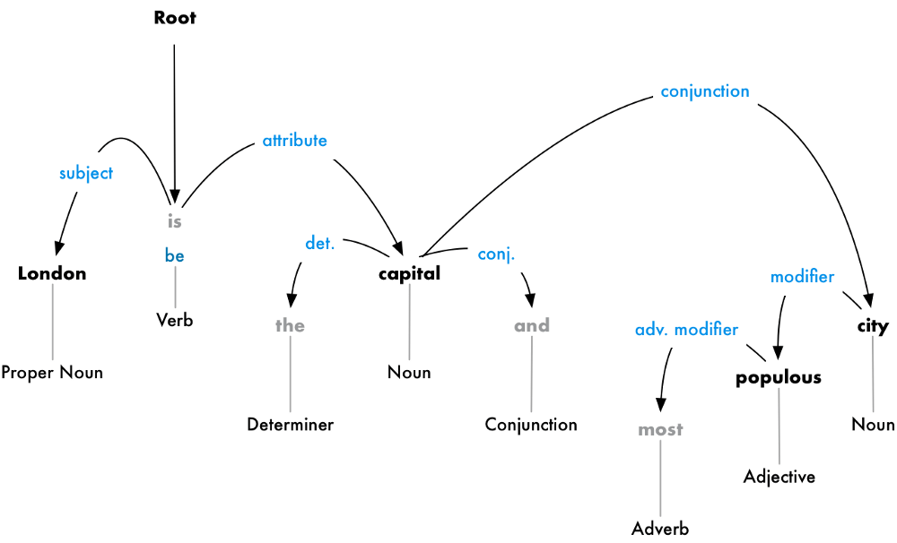
But we can go one step further. In addition to identifying the parent word of each word, we can also predict the type of relationship that exists between those two words:
This parse tree shows us that the subject of the sentence is the noun “London” and it has a “be” relationship with “capital”. We finally know something useful — London is a capital! And if we followed the complete parse tree for the sentence (beyond what is shown), we would even found out that London is the capital of the United Kingdom.
Just like how we predicted parts of speech earlier using a machine learning model, dependency parsing also works by feeding words into a machine learning model and outputting a result. But parsing word dependencies is particularly complex task and would require an entire article to explain in any detail. If you are curious how it works, a great place to start reading is Matthew Honnibal’s excellent article “Parsing English in 500 Lines of Python”.
But despite a note from the author in 2015 saying that this approach is now standard, it’s actually out of date and not even used by the author anymore. In 2016, Google released a new dependency parser called Parsey McParseface which outperformed previous benchmarks using a new deep learning approach which quickly spread throughout the industry. Then a year later, they released an even newer model called ParseySaurus which improved things further. In other words, parsing techniques are still an active area of research and constantly changing and improving.
It’s also important to remember that many English sentences are ambiguous and just really hard to parse. In those cases, the model will make a guess based on what parsed version of the sentence seems most likely but it’s not perfect and sometimes the model will be embarrassingly wrong. But over time our NLP models will continue to get better at parsing text in a sensible way.
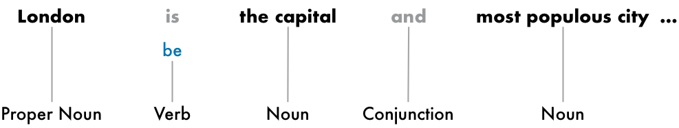
So far, we’ve treated every word in our sentence as a separate entity. But sometimes it makes more sense to group together the words that represent a single idea or thing. We can use the information from the dependency parse tree to automatically group together words that are all talking about the same thing.
For example, instead of this:
We can group the noun phrases to generate this:
Whether or not we do this step depends on our end goal. But it’s often a quick and easy way to simplify the sentence if we don’t need extra detail about which words are adjectives and instead care more about extracting complete ideas.
Step 7: Named Entity Recognition (NER)
Now that we’ve done all that hard work, we can finally move beyond grade-school grammar and start actually extracting ideas.
In our sentence, we have the following nouns:
Some of these nouns present real things in the world. For example, “London”, “England” and “United Kingdom” represent physical places on a map. It would be nice to be able to detect that! With that information, we could automatically extract a list of real-world places mentioned in a document using NLP.
The goal of Named Entity Recognition, or NER, is to detect and label these nouns with the real-world concepts that they represent. Here’s what our sentence looks like after running each token through our NER tagging model:
But NER systems aren’t just doing a simple dictionary lookup. Instead, they are using the context of how a word appears in the sentence and a statistical model to guess which type of noun a word represents. A good NER system can tell the difference between “Brooklyn Decker” the person and the place “Brooklyn” using context clues.
Here are just some of the kinds of objects that a typical NER system can tag:
People’s names
Company names
Geographic locations (Both physical and political)
Product names
Dates and times
Amounts of money
Names of events
NER has tons of uses since it makes it so easy to grab structured data out of text. It’s one of the easiest ways to quickly get value out of an NLP pipeline.
At this point, we already have a useful representation of our sentence. We know the parts of speech for each word, how the words relate to each other and which words are talking about named entities.
However, we still have one big problem. English is full of pronouns — words like he, she, and it. These are shortcuts that we use instead of writing out names over and over in each sentence. Humans can keep track of what these words represent based on context. But our NLP model doesn’t know what pronouns mean because it only examines one sentence at a time.
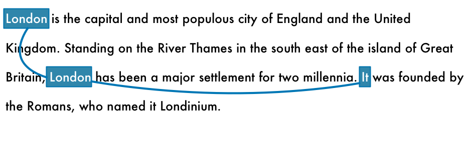
Let’s look at the third sentence in our document:
“It was founded by the Romans, who named it Londinium.”
If we parse this with our NLP pipeline, we’ll know that “it” was founded by Romans. But it’s a lot more useful to know that “London” was founded by Romans.
As a human reading this sentence, you can easily figure out that “it” means “London”. The goal of coreference resolution is to figure out this same mapping by tracking pronouns across sentences. We want to figure out all the words that are referring to the same entity.
Here’s the result of running coreference resolution on our document for the word “London”:
With coreference information combined with the parse tree and named entity information, we should be able to extract a lot of information out of this document!
Coreference resolution is one of the most difficult steps in our pipeline to implement. It’s even more difficult than sentence parsing. Recent advances in deep learning have resulted in new approaches that are more accurate, but it isn’t perfect yet. If you want to learn more about how it works, start here.
Coreference resolution is an optional step that isn’t always done.
Whew, that’s a lot of steps!
Note: Before we continue, it’s worth mentioning that these are the steps in a typical NLP pipeline, but you will skip steps or re-order steps depending on what you want to do and how your NLP library is implemented. For example, some libraries like spaCy do sentence segmentation much later in the pipeline using the results of the dependency parse.
So how do we code this pipeline? Thanks to amazing python libraries like spaCy, it’s already done! The steps are all coded and ready for you to use.
First, assuming you have Python 3 installed already, you can install spaCy like this:
# Install spaCy
pip3 install -U spacy

# Download the large English model for spaCy
python3 -m spacy download en_core_web_lg

# Install textacy which will also be useful
pip3 install -U textacy
Then the code to run an NLP pipeline on a piece of text looks like this:
import spacy

# Load the large English NLP model
nlp = spacy.load('en_core_web_lg')

# The text we want to examine
text = """London is the capital and most populous city of England and
the United Kingdom.  Standing on the River Thames in the south east
of the island of Great Britain, London has been a major settlement
for two millennia. It was founded by the Romans, who named it Londinium.
"""

# Parse the text with spaCy. This runs the entire pipeline.
doc = nlp(text)

# 'doc' now contains a parsed version of text. We can use it to do anything we want!
# For example, this will print out all the named entities that were detected:
for entity in doc.ents:
print(f"{entity.text} ({entity.label_})")
If you run that, you’ll get a list of named entities and entity types detected in our document:
London (GPE)
England (GPE)
the United Kingdom (GPE)
the River Thames (FAC)
Great Britain (GPE)
London (GPE)
two millennia (DATE)
Romans (NORP)
Londinium (PERSON)
Notice that it makes a mistake on “Londinium” and thinks it is the name of a person instead of a place. This is probably because there was nothing in the training data set similar to that and it made a best guess. Named Entity Detection often requires a little bit of model fine tuning if you are parsing text that has unique or specialized terms like this.
Let’s take the idea of detecting entities and twist it around to build a data scrubber. Let’s say you are trying to comply with the new GDPR privacy regulations and you’ve discovered that you have thousands of documents with personally identifiable information in them like people’s names. You’ve been given the task of removing any and all names from your documents.
Going through thousands of documents and trying to redact all the names by hand could take years. But with NLP, it’s a breeze. Here’s a simple scrubber that removes all the names it detects:
import spacy

# Load the large English NLP model
nlp = spacy.load('en_core_web_lg')

# Replace a token with "REDACTED" if it is a name
def replace_name_with_placeholder(token):
    if token.ent_iob != 0 and token.ent_type_ == "PERSON":
        return "[REDACTED] "
    else:
        return token.string

# Loop through all the entities in a document and check if they are names
def scrub(text):
    doc = nlp(text)
    for ent in doc.ents:
        ent.merge()
    tokens = map(replace_name_with_placeholder, doc)
    return "".join(tokens)

s = """
In 1950, Alan Turing published his famous article "Computing Machinery and Intelligence". In 1957, Noam Chomsky’s
Syntactic Structures revolutionized Linguistics with 'universal grammar', a rule based system of syntactic structures.
"""

print(scrub(s))
And if you run that, you’ll see that it works as expected:
In 1950, [REDACTED] published his famous article "Computing Machinery and Intelligence". In 1957, [REDACTED]
Syntactic Structures revolutionized Linguistics with 'universal grammar', a rule based system of syntactic structures.
Extracting Facts
What you can do with spaCy right out of the box is pretty amazing. But you can also use the parsed output from spaCy as the input to more complex data extraction algorithms. There’s a python library called textacy that implements several common data extraction algorithms on top of spaCy. It’s a great starting point.
One of the algorithms it implements is called Semi-structured Statement Extraction. We can use it to search the parse tree for simple statements where the subject is “London” and the verb is a form of “be”. That should help us find facts about London.
Here’s how that looks in code:
import spacy
import textacy.extract

# Load the large English NLP model
nlp = spacy.load('en_core_web_lg')

# The text we want to examine
text = """London is the capital and most populous city of England and  the United Kingdom.
Standing on the River Thames in the south east of the island of Great Britain,
London has been a major settlement  for two millennia.  It was founded by the Romans,
who named it Londinium.
"""

# Parse the document with spaCy
doc = nlp(text)

# Extract semi-structured statements
statements = textacy.extract.semistructured_statements(doc, "London")

# Print the results
print("Here are the things I know about London:")

for statement in statements:
    subject, verb, fact = statement
print(f" - {fact}")
And here’s what it prints:
Here are the things I know about London:
 - the capital and most populous city of England and the United Kingdom.
- a major settlement for two millennia.
Maybe that’s not too impressive. But if you run that same code on the entire London wikipedia article text instead of just three sentences, you’ll get this more impressive result:
Here are the things I know about London:
 - the capital and most populous city of England and the United Kingdom
 - a major settlement for two millennia
 - the world's most populous city from around 1831 to 1925
 - beyond all comparison the largest town in England
 - still very compact
 - the world's largest city from about 1831 to 1925
 - the seat of the Government of the United Kingdom
 - vulnerable to flooding
 - "one of the World's Greenest Cities" with more than 40 percent green space or open water
 - the most populous city and metropolitan area of the European Union and the second most populous in Europe
 - the 19th largest city and the 18th largest metropolitan region in the world
 - Christian, and has a large number of churches, particularly in the City of London
 - also home to sizeable Muslim, Hindu, Sikh, and Jewish communities
 - also home to 42 Hindu temples
 - the world's most expensive office market for the last three years according to world property journal (2015) report
 - one of the pre-eminent financial centres of the world as the most important location for international finance
 - the world top city destination as ranked by TripAdvisor users
 - a major international air transport hub with the busiest city airspace in the world
 - the centre of the National Rail network, with 70 percent of rail journeys starting or ending in London
 - a major global centre of higher education teaching and research and has the largest concentration of higher education institutes in Europe
 - home to designers Vivienne Westwood, Galliano, Stella McCartney, Manolo Blahnik, and Jimmy Choo, among others
 - the setting for many works of literature
 - a major centre for television production, with studios including BBC Television Centre, The Fountain Studios and The London Studios
 - also a centre for urban music
 - the "greenest city" in Europe with 35,000 acres of public parks, woodlands and gardens
 - not the capital of England, as England does not have its own government
Now things are getting interesting! That’s a pretty impressive amount of information we’ve collected automatically.
For extra credit, try installing the neuralcoref library and adding Coreference Resolution to your pipeline. That will get you a few more facts since it will catch sentences that talk about “it” instead of mentioning “London” directly.
What else can we do?
By looking through the spaCy docs and textacy docs, you’ll see lots of examples of the ways you can work with parsed text. What we’ve seen so far is just a tiny sample.
Here’s another practical example: Imagine that you were building a website that let’s the user view information for every city in the world using the information we extracted in the last example.
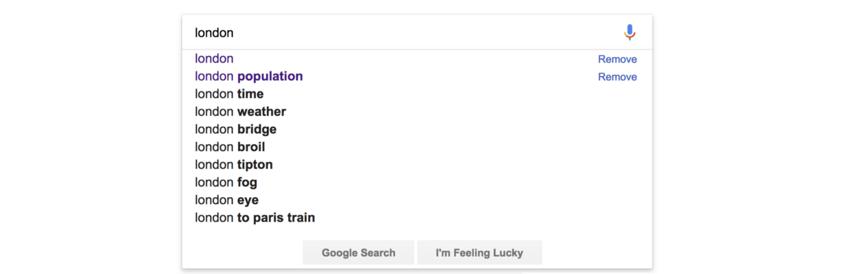
If you had a search feature on the website, it might be nice to autocomplete common search queries like Google does:
But to do this, we need a list of possible completions to suggest to the user. We can use NLP to quickly generate this data.
Here’s one way to extract frequently-mentioned noun chunks from a document:
import spacy
import textacy.extract

# Load the large English NLP model
nlp = spacy.load('en_core_web_lg')

# The text we want to examine
text = """London is [.. shortened for space ..]"""

# Parse the document with spaCy
doc = nlp(text)

# Extract noun chunks that appear
noun_chunks = textacy.extract.noun_chunks(doc, min_freq=3)

# Convert noun chunks to lowercase strings
noun_chunks = map(str, noun_chunks)
noun_chunks = map(str.lower, noun_chunks)

# Print out any nouns that are at least 2 words long
for noun_chunk in set(noun_chunks):
    if len(noun_chunk.split(" ")) > 1:
print(noun_chunk)
If you run that on the London Wikipedia article, you’ll get output like this:
westminster abbey
natural history museum
west end
east end
st paul's cathedral
royal albert hall
london underground
great fire
british museum
london eye
.... etc ....
Going Deeper
This is just a tiny taste of what you can do with NLP. In future posts, we’ll talk about other applications of NLP like Text Classification and how systems like Amazon Alexa parse questions.
But until then, install spaCy and start playing around! Or if you aren’t a Python user and end up using a different NLP library, the ideas should all work roughly the same way.